You can also search not for the best point in the direction of the gradient, but for some one better than the current one.

The easiest to implement of all local optimization methods. It has rather weak convergence conditions, but the rate of convergence is quite low (linear). The gradient method step is often used as part of other optimization methods, such as the Fletcher–Reeves method.

Description [ | ]

Improvements[ | ]

The gradient descent method turns out to be very slow when moving along a ravine, and as the number of variables in the objective function increases, this behavior of the method becomes typical. To combat this phenomenon it is used, the essence of which is very simple. Having made two steps of gradient descent and obtained three points, the third step should be taken in the direction of the vector connecting the first and third points, along the bottom of the ravine.

For functions close to quadratic, the conjugate gradient method is effective.

Application in artificial neural networks[ | ]

The gradient descent method, with some modification, is widely used for perceptron training and is known in the theory of artificial neural networks as the backpropagation method. When training a perceptron-type neural network, it is necessary to change the network's weighting coefficients so as to minimize the average error at the output of the neural network when a sequence of training input data is fed to the input. Formally, in order to take just one step using the gradient descent method (make just one change in the network parameters), it is necessary to sequentially submit absolutely the entire set of training data to the network input, calculate the error for each object of the training data and calculate the necessary correction of the network coefficients (but not do this correction), and after submitting all the data, calculate the amount in the correction of each network coefficient (sum of gradients) and correct the coefficients “one step”. Obviously, with a large set of training data, the algorithm will work extremely slowly, so in practice, network coefficients are often adjusted after each training element, where the gradient value is approximated by the gradient of the cost function, calculated on only one training element. This method is called stochastic gradient descent or operational gradient descent . Stochastic gradient descent is a form of stochastic approximation. The theory of stochastic approximations provides conditions for the convergence of the stochastic gradient descent method.

Links [ | ]

• J. Mathews. Module for Steepest Descent or Gradient Method. (unavailable link)

Literature [ | ]

• Akulich I. L. Mathematical programming in examples and problems. - M.: Higher School, 1986. - P. 298-310.
• Gill F., Murray W., Wright M. Practical optimization = Practical Optimization. - M.: Mir, 1985.
• Korshunov Yu. M., Korshunov Yu. M. Mathematical foundations of cybernetics. - M.: Energoatomizdat, 1972.
• Maksimov Yu. A., Fillipovskaya E. A. Algorithms for solving nonlinear programming problems. - M.: MEPhI, 1982.
• Maksimov Yu. A. Algorithms for linear and discrete programming. - M.: MEPhI, 1980.
• Korn G., Korn T. Handbook of mathematics for scientists and engineers. - M.: Nauka, 1970. - P. 575-576.
• S. Yu. Gorodetsky, V. A. Grishagin. Nonlinear programming and multiextremal optimization. - Nizhny Novgorod: Nizhny Novgorod University Publishing House, 2007. - P. 357-363.

The gradient of the differentiable function f(x) at the point X called n-dimensional vector f(x) , whose components are partial derivatives of the function f(x), calculated at the point X, i.e.

f"(x ) = (df(x)/dh 1 , …, df(x)/dx n) T .

This vector is perpendicular to the plane through the point X, and tangent to the level surface of the function f(x), passing through a point X.At each point of such a surface the function f(x) takes the same value. Equating the function to various constant values ​​C 0 , C 1 , ..., we obtain a series of surfaces characterizing its topology (Fig. 2.8).

The gradient vector is directed towards the fastest increase in the function at a given point. Vector opposite to gradient (-f’(x)) , called anti-gradient and is directed towards the fastest decrease of the function. At the minimum point, the gradient of the function is zero. First-order methods, also called gradient and minimization methods, are based on the properties of gradients. Using these methods in the general case allows you to determine the local minimum point of a function.

Obviously, if there is no additional information, then from the starting point X it is reasonable to go to the point X, lying in the direction of the antigradient - the fastest decrease of the function. Choosing as the direction of descent r[k] anti-gradient - f'(x[k] ) at the point X[k], we obtain an iterative process of the form

X[ k+ 1] = x[k]-a k f"(x[k] ) , and k > 0; k=0, 1, 2, ...

In coordinate form, this process is written as follows:

x i [ k+1]=x i[k] - a kf(x[k] ) /x i

i = 1, ..., n; k= 0, 1, 2,...

As a criterion for stopping the iterative process, either the fulfillment of the condition of small increment of the argument || x[k+l] -x[k] || <= e , либо выполнение условия малости градиента

|| f'(x[k+l] ) || <= g ,

Here e and g are given small quantities.

A combined criterion is also possible, consisting in the simultaneous fulfillment of the specified conditions. Gradient methods differ from each other in the way they choose the step size and k.

In the method with a constant step, a certain constant step value is selected for all iterations. Quite a small step and k will ensure that the function decreases, i.e., the inequality

f(x[ k+1]) = f(x[k] – a k f’(x[k] )) < f(x[k] ) .

However, this may lead to the need to carry out an unacceptably large number of iterations to reach the minimum point. On the other hand, a step that is too large can cause an unexpected increase in the function or lead to oscillations around the minimum point (cycling). Due to the difficulty of obtaining the necessary information to select the step size, methods with constant steps are rarely used in practice.

Gradient ones are more economical in terms of the number of iterations and reliability variable step methods, when, depending on the results of calculations, the step size changes in some way. Let us consider the variants of such methods used in practice.

When using the steepest descent method at each iteration, the step size and k is selected from the minimum condition of the function f(x) in the direction of descent, i.e.
f(x[k]–a k f’(x[k])) = f(x[k] – af"(x[k])) .

This condition means that movement along the antigradient occurs as long as the value of the function f(x) decreases. From a mathematical point of view, at each iteration it is necessary to solve the problem of one-dimensional minimization according to A functions
j (a) = f(x[k]-af"(x[k])) .

The algorithm of the steepest descent method is as follows.

1. Set the coordinates of the starting point X.

2. At the point X[k], k = 0, 1, 2, ... calculates the gradient value f'(x[k]) .

3. The step size is determined a k, by one-dimensional minimization over A functions j (a) = f(x[k]-af"(x[k])).

4. The coordinates of the point are determined X[k+ 1]:

x i [ k+ 1]= xi[k]– a k f’ i (x[k]), i = 1,..., p.

5. The conditions for stopping the steration process are checked. If they are fulfilled, then the calculations stop. Otherwise, go to step 1.

In the method under consideration, the direction of movement from the point X[k] touches the level line at the point x[k+ 1] (Fig. 2.9). The descent trajectory is zigzag, with adjacent zigzag links orthogonal to each other. Indeed, a step a k is chosen by minimizing by A functions? (a) = f(x[k] -af"(x[k])) . Necessary condition for the minimum of a function d j (a)/da = 0. Having calculated the derivative of a complex function, we obtain the condition for the orthogonality of the vectors of descent directions at neighboring points:

dj (a)/da = -f’(x[k+ 1]f'(x[k]) = 0.

Gradient methods converge to a minimum at high speed (geometric progression speed) for smooth convex functions. Such functions have the greatest M and least m eigenvalues ​​of the matrix of second derivatives (Hessian matrix)

differ little from each other, i.e. matrix N(x) well conditioned. Recall that the eigenvalues ​​l i, i =1, …, n, the matrices are the roots of the characteristic equation

However, in practice, as a rule, the functions being minimized have ill-conditioned matrices of second derivatives (t/m<< 1). The values ​​of such functions along some directions change much faster (sometimes by several orders of magnitude) than in other directions. Their level surfaces in the simplest case are strongly elongated (Fig. 2.10), and in more complex cases they bend and look like ravines. Functions with such properties are called gully. The direction of the antigradient of these functions (see Fig. 2.10) deviates significantly from the direction to the minimum point, which leads to a slowdown in the speed of convergence.

The convergence rate of gradient methods also depends significantly on the accuracy of gradient calculations. Loss of accuracy, which usually occurs in the vicinity of minimum points or in a gully situation, can generally disrupt the convergence of the gradient descent process. Due to the above reasons, gradient methods are often used in combination with other, more effective methods at the initial stage of solving a problem. In this case, the point X is far from the minimum point, and steps in the direction of the antigradient make it possible to achieve a significant decrease in the function.

The gradient methods discussed above find the minimum point of a function in the general case only in an infinite number of iterations. The conjugate gradient method generates search directions that are more consistent with the geometry of the function being minimized. This significantly increases the speed of their convergence and allows, for example, to minimize the quadratic function

f(x) = (x, Hx) + (b, x) + a

with a symmetric positive definite matrix N in a finite number of steps p, equal to the number of function variables. Any smooth function in the vicinity of the minimum point can be well approximated by a quadratic function, therefore conjugate gradient methods are successfully used to minimize non-quadratic functions. In this case, they cease to be finite and become iterative.

By definition, two n-dimensional vector X And at called conjugated relative to the matrix H(or H-conjugate), if the scalar product (x, Well) = 0. Here N - symmetric positive definite matrix of size n X p.

One of the most significant problems in conjugate gradient methods is the problem of efficiently constructing directions. The Fletcher-Reeves method solves this problem by transforming the antigradient at each step -f(x[k]) in the direction p[k], H-conjugate with previously found directions r, r, ..., r[k-1]. Let us first consider this method in relation to the problem of minimizing a quadratic function.

Directions r[k] is calculated using the formulas:

p[ k] = -f'(x[k]) +b k-1 p[k-l], k>= 1;

p = - f’(x) .

b values k-1 are chosen so that the directions p[k], r[k-1] were H-conjugate :

(p[k], HP[k- 1])= 0.

As a result, for the quadratic function

,

the iterative minimization process has the form

x[ k+l] =x[k]+a k p[k],

Where r[k] - direction of descent to k- m step; and k - step size. The latter is selected from the minimum condition of the function f(x) By A in the direction of movement, i.e. as a result of solving the one-dimensional minimization problem:

f(x[ k] + a k r[k]) = f(x[k] + ar [k]) .

For a quadratic function

The algorithm of the Fletcher-Reeves conjugate gradient method is as follows.

1. At the point X calculated p = -f'(x) .

2. On k- m step, using the above formulas, the step is determined A k . and period X[k+ 1].

3. Values ​​are calculated f(x[k+1]) And f'(x[k+1]) .

4. If f'(x) = 0, then point X[k+1] is the minimum point of the function f(x). Otherwise, a new direction is determined p[k+l] from the relation

and the transition to the next iteration is carried out. This procedure will find the minimum of a quadratic function in no more than n steps. When minimizing non-quadratic functions, the Fletcher-Reeves method becomes iterative from finite. In this case, after (p+ 1)th iteration of procedure 1-4 are repeated cyclically with replacement X on X[n+1] , and calculations end at , where is a given number. In this case, the following modification of the method is used:

x[ k+l] = x[k]+a k p[k],

p[ k] = -f’(x[k])+ b k- 1 p[k-l], k>= 1;

p = -f’( x);

f(x[ k] + a k p[k]) = f(x[k] +ap[k];

.

Here I- many indexes: I= (0, n, 2 p, salary, ...), i.e. the method is updated every n steps.

The geometric meaning of the conjugate gradient method is as follows (Fig. 2.11). From a given starting point X descent is carried out in the direction r = -f"(x). At the point X the gradient vector is determined f"(x). Because X is the minimum point of the function in the direction r, That f'(x) orthogonal to vector r. Then the vector is found r , H-conjugate to r. Next, we find the minimum of the function along the direction r etc.

Conjugate direction methods are among the most effective for solving minimization problems. However, it should be noted that they are sensitive to errors that occur during the counting process. With a large number of variables, the error can increase so much that the process will have to be repeated even for a quadratic function, i.e. the process for it does not always fit into n steps.

The steepest descent method is a gradient method with a variable step. At each iteration, the step size k is selected from the condition of the minimum of the function f(x) in the direction of descent, i.e.

This condition means that movement along the antigradient occurs as long as the value of the function f (x) decreases. From a mathematical point of view, at each iteration it is necessary to solve the problem of one-dimensional minimization by function

()=f (x (k) -f (x (k)))

Let's use the golden ratio method for this.

The algorithm of the steepest descent method is as follows.

The coordinates of the starting point x (0) are specified.

At point x (k) , k = 0, 1, 2, ..., the gradient value f (x (k)) is calculated.

The step size k is determined by one-dimensional minimization using the function

()=f (x (k) -f (x (k))).

The coordinates of the point x (k) are determined:

x i (k+1) = x i (k) - k f i (x (k)), i=1, …, n.

The condition for stopping the iterative process is checked:

||f (x (k +1))|| .

If it is fulfilled, then the calculations stop. Otherwise, we proceed to step 1. The geometric interpretation of the steepest descent method is presented in Fig. 1.

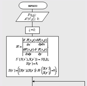
Rice. 2.1. Block diagram of the steepest descent method.

Implementation of the method in the program:

Method of steepest descent.

Rice. 2.2. Implementation of the steepest descent method.

Conclusion: In our case, the method converged in 7 iterations. Point A7 (0.6641; -1.3313) is an extremum point. Method of conjugate directions. For quadratic functions, you can create a gradient method in which the convergence time will be finite and equal to the number of variables n.

Let us call a certain direction and conjugate with respect to some positive definite Hess matrix H if:

Then i.e. So for unit H, the conjugate direction means their perpendicular. In the general case, H is non-trivial. In the general case, conjugacy is the application of the Hess matrix to a vector - it means rotating this vector by some angle, stretching or compressing it.

And now the vector is orthogonal, i.e. conjugacy is not the orthogonality of the vector, but the orthogonality of the rotated vector.e.i.

Rice. 2.3. Block diagram of the conjugate directions method.

Implementation of the method in the program: Method of conjugate directions.

Rice. 2.4. Implementation of the conjugate directions method.

Rice. 2.5. Graph of the conjugate directions method.

Conclusion: Point A3 (0.6666; -1.3333) was found in 3 iterations and is an extremum point.

3. Analysis of methods for determining the minimum and maximum value of a function in the presence of restrictions

Recall that a general constrained optimization problem looks like this:

f(x) ® min, x О W,

where W is a proper subset of R m. A subclass of problems with equality-type constraints is distinguished by the fact that the set  is defined by constraints of the form

f i (x) = 0, where f i: R m ®R (i = 1, …, k).

Thus,W = (x О R m: f i (x) = 0, i = 1, …, k).

It will be convenient for us to write index "0" for the function f. Thus, the optimization problem with equality type constraints is written as

f 0 (x) ® min, (3.1)

f i (x) = 0, i = 1, …, k. (3.2)

If we now denote by f a function on R m with values ​​in R k, the coordinate notation of which has the form f(x) = (f 1 (x), ..., f k (x)), then (3.1)–(3.2) we can also write it in the form

f 0 (x) ® min, f(x) = Q.

Geometrically, a problem with equality type constraints is a problem of finding the lowest point of the graph of a function f 0 over the manifold  (see Fig. 3.1).

Points that satisfy all the constraints (i.e., points in the set ) are usually called admissible. An admissible point x* is called a conditional minimum of the function f 0 under the constraints f i (x) = 0, i = 1, ..., k (or a solution to problem (3.1)–(3.2)), if for all admissible points x f 0 (x *)  f 0 (x). (3.3)

If (3.3) is satisfied only for admissible x lying in some neighborhood V x * of point x*, then we speak of a local conditional minimum. The concepts of conditional strict local and global minima are defined in a natural way.

Example 6.8.3-1. Find the minimum of the function Q(x,y) using the GDS method.

Let Q(x,y) = x 2 +2y 2 ; x 0 = 2;y 0 = 1.

Let us check the sufficient conditions for the existence of a minimum:

Let's do one iteration according to the algorithm.

1. Q(x 0 ,y 0) = 6.

2. For x = x 0 and y = y 0,

3. Step l k = l 0 = 0.5

So 4< 8, следовательно, условие сходимости не выполняется и требуется, уменьшив шаг (l=l /2), повторять п.п.3-4 до выполнения условия сходимости. То есть, полученный шаг используется для нахождения следующей точки траектории спуска.

The essence of the method is as follows. From the selected point (x 0 ,y 0) the descent is carried out in the direction of the antigradient until the minimum value of the objective function Q(x, y) along the ray is reached (Fig. 6.8.4-1). At the found point, the beam touches the level line. Then, from this point, the descent is carried out in the direction of the antigradient (perpendicular to the level line) until the corresponding ray touches the level line passing through it at a new point, etc.

Let us express the objective function Q(x, y) in terms of step l. In this case, we present the target function at a certain step as a function of one variable, i.e. step size

The step size at each iteration is determined from the minimum condition:

Min( (l)) l k = l*(x k , y k), l >0.

Thus, at each iteration, the choice of step l k involves solving a one-dimensional optimization problem. According to the method of solving this problem, they are distinguished:

· analytical method (NAA);

· numerical method (NMS).

In the NSA method, the step value is obtained from the condition, and in the NSF method, the value l k is found on a segment with a given accuracy using one of the one-dimensional optimization methods.

Example 6.8.4-1. Find the minimum of the function Q(x,y)=x 2 + 2y 2 with an accuracy of e=0.1, under initial conditions: x 0 =2; y 0 =1.

Let's do one iteration using the method NSA.

=(x-2lx) 2 +2(y-4ly) 2 = x 2 -4lx 2 +4l 2 x 2 +2y 2 -16ly 2 +32l 2 y 2 .

From the condition ¢(l)=0 we find the value of l*:

The resulting function l=l(x,y) allows you to find the value of l. For x=2 and y=1 we have l=0.3333.

Let's calculate the coordinates of the next point:

Let's check the fulfillment of the criterion for ending iterations at k=1:

Since |2*0.6666|>0.1 and |-0.3333*4|>0.1, then the conditions for ending the iteration process are not met, i.e. minimum not found. Therefore, you should calculate the new value of l for x=x 1 and y=y 1 and obtain the coordinates of the next descent point. Calculations continue until the descent termination conditions are met.

The difference between the numerical NN method and the analytical one is that the search for the value of l at each iteration occurs using one of the numerical methods of one-dimensional optimization (for example, the dichotomy method or the golden section method). In this case, the range of permissible values ​​l - serves as the uncertainty interval.

Fig.3. Geometric interpretation of the steepest descent method. At each step, it is chosen so that the next iteration is the minimum point of the function on the ray L.

This version of the gradient method is based on the choice of step from the following considerations. From the point we will move in the direction of the antigradient until we reach the minimum of the function f in this direction, i.e. on the ray:

In other words, it is chosen so that the next iteration is the minimum point of the function f on the ray L (see Fig. 3). This version of the gradient method is called the steepest descent method. Note, by the way, that in this method the directions of adjacent steps are orthogonal.

The steepest descent method requires solving a one-dimensional optimization problem at each step. Practice shows that this method often requires fewer operations than the gradient method with a constant step.

In the general situation, however, the theoretical convergence rate of the steepest descent method is no higher than the convergence rate of the gradient method with a constant (optimal) step.

Numerical examples

Gradient descent method with constant step

To study the convergence of the gradient descent method with a constant step, the function was chosen:

From the results obtained, we can conclude that if the gap is too large, the method diverges; if the gap is too small, it converges slowly and the accuracy is worse. It is necessary to choose the largest step from those at which the method converges.

Gradient method with step division

To study the convergence of the gradient descent method with step division (2), the function was chosen:

The initial approximation is point (10,10).

Stopping criterion used:

The results of the experiment are shown in the table:

From the results obtained, we can conclude about the optimal choice of parameters: , although the method is not very sensitive to the choice of parameters.

Method of steepest descent

To study the convergence of the steepest descent method, the following function was chosen:

The initial approximation is point (10,10). Stopping criterion used:

To solve one-dimensional optimization problems, the golden section method was used.

The method achieved an accuracy of 6e-8 in 9 iterations.

From this we can conclude that the steepest descent method converges faster than the step-split gradient method and the constant-step gradient descent method.

The disadvantage of the steepest descent method is that it requires solving a one-dimensional optimization problem.

When programming gradient descent methods, you should be careful when choosing parameters, namely

• · Gradient descent method with a constant step: the step should be chosen less than 0.01, otherwise the method diverges (the method may diverge even with such a step, depending on the function being studied).
• · The gradient method with step division is not very sensitive to the choice of parameters. One of the options for selecting parameters:
• · Steepest descent method: The golden ratio method (when applicable) can be used as a one-dimensional optimization method.

The conjugate gradient method is an iterative method for unconditional optimization in a multidimensional space. The main advantage of the method is that it solves a quadratic optimization problem in a finite number of steps. Therefore, first the conjugate gradient method for optimizing the quadratic functional is described, iterative formulas are derived, and estimates of the convergence rate are given. After this, it is shown how the adjoint method is generalized to optimize an arbitrary functional, various variants of the method are considered, and convergence is discussed.

Statement of the optimization problem

Let a set be given and an objective function defined on this set. The optimization problem consists of finding the exact upper or exact lower bound of the objective function on the set. The set of points at which the lower bound of the objective function is reached is designated.

If, then the optimization problem is called unconstrained. If, then the optimization problem is called constrained.

Conjugate gradient method for quadratic functional

Statement of the method

Consider the following optimization problem:

Here is a symmetric positive definite size matrix. This optimization problem is called quadratic. Note that. The condition for an extremum of a function is equivalent to the system The function reaches its lower bound at a single point defined by the equation. Thus, this optimization problem is reduced to solving a system of linear equations. The idea of ​​the conjugate gradient method is as follows: Let be the basis in. Then for any point the vector is expanded into the basis. Thus, it can be represented in the form

Each subsequent approximation is calculated using the formula:

Definition. Two vectors and are said to be conjugate with respect to the symmetric matrix B if

Let us describe the method of constructing a basis in the conjugate gradient method. We choose an arbitrary vector as an initial approximation. At each iteration the following rules are selected:

Basis vectors are calculated using the formulas:

The coefficients are chosen so that the vectors and are conjugate with respect to A.

If we denote by , then after several simplifications we obtain the final formulas used when applying the conjugate gradient method in practice:

For the conjugate gradient method, the following theorem holds: Theorem Let, where is a symmetric positive definite matrix of size. Then the conjugate gradient method converges in no more than steps and the following relations hold:

Convergence of the method

If all calculations are accurate and the initial data are accurate, then the method converges to solving the system in no more than iterations, where is the dimension of the system. A more refined analysis shows that the number of iterations does not exceed, where is the number of different eigenvalues ​​of the matrix A. To estimate the rate of convergence, the following (rather rough) estimate is correct:

It allows you to estimate the rate of convergence if estimates for the maximum and minimum eigenvalues ​​of the matrix are known. In practice, the following stopping criterion is most often used:

Computational complexity

At each iteration of the method, operations are performed. This number of operations is required to calculate the product - this is the most time-consuming procedure at each iteration. Other calculations require O(n) operations. The total computational complexity of the method does not exceed - since the number of iterations is no more than n.

Numerical example

Let us apply the conjugate gradient method to solve a system where, using the conjugate gradient method, the solution to this system is obtained in two iterations. The eigenvalues ​​of the matrix are 5, 5, -5 - among them there are two different ones, therefore, according to the theoretical estimate, the number of iterations could not exceed two

The conjugate gradient method is one of the most effective methods for solving SLAEs with a positive definite matrix. The method guarantees convergence in a finite number of steps, and the required accuracy can be achieved much earlier. The main problem is that due to the accumulation of errors, the orthogonality of the basis vectors may be violated, which impairs the convergence

The conjugate gradient method in general

Let us now consider a modification of the conjugate gradient method for the case when the minimized functional is not quadratic: We will solve the problem:

Continuously differentiable function. To modify the conjugate gradient method to solve this problem, it is necessary to obtain for formulas that do not include matrix A:

can be calculated using one of three formulas:

1. - Fletcher-Reeves method

• 2. - Polak-Ribi`ere method

If the function is quadratic and strictly convex, then all three formulas give the same result. If is an arbitrary function, then each of the formulas corresponds to its own modification of the conjugate gradient method. The third formula is rarely used because it requires the function and the calculation of the Hessian of the function at each step of the method.

If the function is not quadratic, the conjugate gradient method may not converge in a finite number of steps. Moreover, accurate calculation at each step is only possible in rare cases. Therefore, the accumulation of errors leads to the fact that the vectors no longer indicate the direction of decrease of the function. Then at some step they believe. The set of all numbers at which it is accepted will be denoted by. The numbers are called method update moments. In practice, it is often chosen where is the dimension of space.

Convergence of the method

For the Fletcher-Reeves method, there is a convergence theorem that imposes not too strict conditions on the function being minimized: Theorem. Let the following conditions be satisfied:

Variety is limited

The derivative satisfies the Lipschitz condition with a constant in some neighborhood

sets M: .

For the Polak-Reiber method, convergence is proven under the assumption that is a strictly convex function. In the general case, it is impossible to prove the convergence of the Polak-Reiber method. On the contrary, the following theorem is true: Theorem. Let us assume that in the Polak-Reiber method the values ​​at each step are calculated exactly. Then there is a function, and an initial guess, such that.

However, in practice the Polak-Reiber method works better. The most common stopping criteria in practice: The gradient norm becomes less than a certain threshold The value of the function has remained almost unchanged for m consecutive iterations

Computational complexity

At each iteration of the Polak-Reiber or Fletcher-Reeves methods, the function and its gradient are calculated once, and the one-dimensional optimization problem is solved. Thus, the complexity of one step of the conjugate gradient method is of the same order of magnitude as the complexity of one step of the steepest descent method. In practice, the conjugate gradient method shows the best convergence speed.

We will search for the minimum of the function using the conjugate gradient method

The minimum of this function is 1 and is reached at point (5, 4). Using this function as an example, let us compare the Polak-Reiber and Fletcher-Reeves methods. Iterations in both methods stop when the squared norm of the gradient becomes smaller at the current step. The golden ratio method is used for selection

Two versions of the conjugate gradient method have been implemented: for minimizing a quadratic functional, and for minimizing an arbitrary function. In the first case, the method is implemented by the vector function FindSolution(matrix A,vector b) Here A and b are the matrix and vector involved in the definition of the quadratic optimization problem. To minimize arbitrary functionality, you can use one of two functions: vector FletcherRievesMethod(int spaceSize, Function F, vector (*GradF) (vector )) vector PolakRibiereMethod(int spaceSize, Function F, vector (*GradF) (vector )) The parameters for both functions are the same and have the following meaning: spaceSize - the dimension of the space (the number of variables on which the minimized functional depends) F - a pointer to the function to be minimized. The function must be of the form double<имя функции>(vector ) GradF - pointer to a function that calculates the gradient of the functional being minimized. Both methods use an auxiliary function to solve a one-dimensional optimization problem. The program implements one-dimensional optimization using the golden section method.

Gradient descent methods are quite powerful tools for solving optimization problems. The main disadvantage of the methods is the limited range of applicability. The conjugate gradient method uses information only about the linear part of the increment at a point, as in gradient descent methods. Moreover, the conjugate gradient method allows you to solve quadratic problems in a finite number of steps. On many other problems, the conjugate gradient method also outperforms the gradient descent method. The convergence of the gradient method depends significantly on how accurately the one-dimensional optimization problem is solved. Possible method loops are resolved using updates. However, if a method gets into a local minimum of a function, it most likely will not be able to escape from it.