The formula for the second remarkable limit is lim x → ∞ 1 + 1 x x = e. Another form of writing looks like this: lim x → 0 (1 + x) 1 x = e.

When we talk about the second remarkable limit, we have to deal with uncertainty of the form 1 ∞, i.e. unity to an infinite degree.

Yandex.RTB R-A-339285-1

Let's consider problems in which the ability to calculate the second remarkable limit will be useful.

Example 1

Find the limit lim x → ∞ 1 - 2 x 2 + 1 x 2 + 1 4 .

Solution

Let's substitute the required formula and perform the calculations.

lim x → ∞ 1 - 2 x 2 + 1 x 2 + 1 4 = 1 - 2 ∞ 2 + 1 ∞ 2 + 1 4 = 1 - 0 ∞ = 1 ∞

Our answer turned out to be one to the power of infinity. To determine the solution method, we use the uncertainty table. Let's choose the second remarkable limit and make a change of variables.

t = - x 2 + 1 2 ⇔ x 2 + 1 4 = - t 2

If x → ∞, then t → - ∞.

Let's see what we got after the replacement:

lim x → ∞ 1 - 2 x 2 + 1 x 2 + 1 4 = 1 ∞ = lim x → ∞ 1 + 1 t - 1 2 t = lim t → ∞ 1 + 1 t t - 1 2 = e - 1 2

Answer: lim x → ∞ 1 - 2 x 2 + 1 x 2 + 1 4 = e - 1 2 .

Example 2

Calculate the limit lim x → ∞ x - 1 x + 1 x .

Solution

Let's substitute infinity and get the following.

lim x → ∞ x - 1 x + 1 x = lim x → ∞ 1 - 1 x 1 + 1 x x = 1 - 0 1 + 0 ∞ = 1 ∞

In the answer, we again got the same thing as in the previous problem, therefore, we can again use the second wonderful limit. Next, we need to select the whole part at the base of the power function:

x - 1 x + 1 = x + 1 - 2 x + 1 = x + 1 x + 1 - 2 x + 1 = 1 - 2 x + 1

After this, the limit takes the following form:

lim x → ∞ x - 1 x + 1 x = 1 ∞ = lim x → ∞ 1 - 2 x + 1 x

Replace variables. Let's assume that t = - x + 1 2 ⇒ 2 t = - x - 1 ⇒ x = - 2 t - 1 ; if x → ∞, then t → ∞.

After that, we write down what we got in the original limit:

lim x → ∞ x - 1 x + 1 x = 1 ∞ = lim x → ∞ 1 - 2 x + 1 x = lim x → ∞ 1 + 1 t - 2 t - 1 = = lim x → ∞ 1 + 1 t - 2 t 1 + 1 t - 1 = lim x → ∞ 1 + 1 t - 2 t lim x → ∞ 1 + 1 t - 1 = = lim x → ∞ 1 + 1 t t - 2 1 + 1 ∞ = e - 2 · (1 + 0) - 1 = e - 2

To perform this transformation, we used the basic properties of limits and powers.

Answer: lim x → ∞ x - 1 x + 1 x = e - 2 .

Example 3

Calculate the limit lim x → ∞ x 3 + 1 x 3 + 2 x 2 - 1 3 x 4 2 x 3 - 5 .

Solution

lim x → ∞ x 3 + 1 x 3 + 2 x 2 - 1 3 x 4 2 x 3 - 5 = lim x → ∞ 1 + 1 x 3 1 + 2 x - 1 x 3 3 2 x - 5 x 4 = = 1 + 0 1 + 0 - 0 3 0 - 0 = 1 ∞

After that, we need to transform the function to apply the second great limit. We got the following:

lim x → ∞ x 3 + 1 x 3 + 2 x 2 - 1 3 x 4 2 x 3 - 5 = 1 ∞ = lim x → ∞ x 3 - 2 x 2 - 1 - 2 x 2 + 2 x 3 + 2 x 2 - 1 3 x 4 2 x 3 - 5 = = lim x → ∞ 1 + - 2 x 2 + 2 x 3 + 2 x 2 - 1 3 x 4 2 x 3 - 5

lim x → ∞ 1 + - 2 x 2 + 2 x 3 + 2 x 2 - 1 3 x 4 2 x 3 - 5 = lim x → ∞ 1 + - 2 x 2 + 2 x 3 + 2 x 2 - 1 x 3 + 2 x 2 - 1 - 2 x 2 + 2 - 2 x 2 + 2 x 3 + 2 x 2 - 1 3 x 4 2 x 3 - 5 = = lim x → ∞ 1 + - 2 x 2 + 2 x 3 + 2 x 2 - 1 x 3 + 2 x 2 - 1 - 2 x 2 + 2 - 2 x 2 + 2 x 3 + 2 x 2 - 1 3 x 4 2 x 3 - 5

Since we now have the same exponents in the numerator and denominator of the fraction (equal to six), the limit of the fraction at infinity will be equal to the ratio of these coefficients at higher powers.

lim x → ∞ 1 + - 2 x 2 + 2 x 3 + 2 x 2 - 1 x 3 + 2 x 2 - 1 - 2 x 2 + 2 - 2 x 2 + 2 x 3 + 2 x 2 - 1 3 x 4 2 x 3 - 5 = = lim x → ∞ 1 + - 2 x 2 + 2 x 3 + 2 x 2 - 1 x 3 + 2 x 2 - 1 - 2 x 2 + 2 - 6 2 = lim x → ∞ 1 + - 2 x 2 + 2 x 3 + 2 x 2 - 1 x 3 + 2 x 2 - 1 - 2 x 2 + 2 - 3

By substituting t = x 2 + 2 x 2 - 1 - 2 x 2 + 2 we get a second remarkable limit. This means that:

lim x → ∞ 1 + - 2 x 2 + 2 x 3 + 2 x 2 - 1 x 3 + 2 x 2 - 1 - 2 x 2 + 2 - 3 = lim x → ∞ 1 + 1 t t - 3 = e - 3

Answer: lim x → ∞ x 3 + 1 x 3 + 2 x 2 - 1 3 x 4 2 x 3 - 5 = e - 3 .

Conclusions

Uncertainty 1 ∞, i.e. unity to an infinite power is a power-law uncertainty, therefore, it can be revealed using the rules for finding the limits of exponential power functions.

If you notice an error in the text, please highlight it and press Ctrl+Enter

From the above article you can find out what the limit is and what it is eaten with - this is VERY important. Why? You may not understand what determinants are and successfully solve them; you may not understand at all what a derivative is and find them with an “A”. But if you don’t understand what a limit is, then solving practical tasks will be difficult. It would also be a good idea to familiarize yourself with the sample solutions and my design recommendations. All information is presented in a simple and accessible form.

And for the purposes of this lesson we will need the following teaching materials: Wonderful Limits And Trigonometric formulas. They can be found on the page. It is best to print out the manuals - it is much more convenient, and besides, you will often have to refer to them offline.

What is so special about remarkable limits? The remarkable thing about these limits is that they were proven by the greatest minds of famous mathematicians, and grateful descendants do not have to suffer from terrible limits with a pile of trigonometric functions, logarithms, powers. That is, when finding the limits, we will use ready-made results that have been proven theoretically.

There are several wonderful limits, but in practice, in 95% of cases, part-time students have two wonderful limits: The first wonderful limit, Second wonderful limit. It should be noted that these are historically established names, and when, for example, they talk about “the first remarkable limit,” they mean by this a very specific thing, and not some random limit taken from the ceiling.

The first wonderful limit

Consider the following limit: (instead of the native letter “he” I will use the Greek letter “alpha”, this is more convenient from the point of view of presenting the material).

According to our rule for finding limits (see article Limits. Examples of solutions) we try to substitute zero into the function: in the numerator we get zero (the sine of zero is zero), and in the denominator, obviously, there is also zero. Thus, we are faced with an uncertainty of the form, which, fortunately, does not need to be disclosed. In the course of mathematical analysis, it is proven that:

This mathematical fact is called The first wonderful limit. I won’t give an analytical proof of the limit, but we’ll look at its geometric meaning in the lesson about infinitesimal functions.

Often in practical tasks functions can be arranged differently, this does not change anything:

- the same first wonderful limit.

But you cannot rearrange the numerator and denominator yourself! If a limit is given in the form , then it must be solved in the same form, without rearranging anything.

In practice, not only a variable, but also an elementary function or a complex function can act as a parameter. The only important thing is that it tends to zero.

Examples:
, , ,

Here , , , , and everything is good - the first wonderful limit is applicable.

But the following entry is heresy:

Why? Because the polynomial does not tend to zero, it tends to five.

By the way, a quick question: what is the limit? ? The answer can be found at the end of the lesson.

In practice, not everything is so smooth; almost never a student is offered to solve a free limit and get an easy pass. Hmmm... I’m writing these lines, and a very important thought came to mind - after all, it’s better to remember “free” mathematical definitions and formulas by heart, this can provide invaluable help in the test, when the question will be decided between “two” and “three”, and the teacher decides to ask the student some simple question or offer to solve a simple example (“maybe he/she still knows what?!”).

Let's move on to consider practical examples:

Example 1

Find the limit

If we notice a sine in the limit, then this should immediately lead us to think about the possibility of applying the first remarkable limit.

First, we try to substitute 0 into the expression under the limit sign (we do this mentally or in a draft):

So we have an uncertainty of the form be sure to indicate in making a decision. The expression under the limit sign is similar to the first wonderful limit, but this is not exactly it, it is under the sine, but in the denominator.

In such cases, we need to organize the first remarkable limit ourselves, using an artificial technique. The line of reasoning could be as follows: “under the sine we have , which means that we also need to get in the denominator.”
And this is done very simply:

That is, the denominator is artificially multiplied in this case by 7 and divided by the same seven. Now our recording has taken on a familiar shape.
When the task is drawn up by hand, it is advisable to mark the first remarkable limit with a simple pencil:

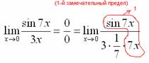
What happened? In fact, our circled expression turned into a unit and disappeared in the work:

Now all that remains is to get rid of the three-story fraction: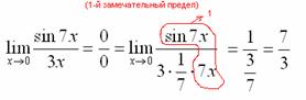

Who has forgotten the simplification of multi-level fractions, please refresh the material in the reference book Hot formulas for school mathematics course .

Ready. Final answer:

If you don’t want to use pencil marks, then the solution can be written like this:

“

Let's use the first wonderful limit

“

Example 2

Find the limit

Again we see a fraction and a sine in the limit. Let’s try to substitute zero into the numerator and denominator:

Indeed, we have uncertainty and, therefore, we need to try to organize the first wonderful limit. In class Limits. Examples of solutions we considered the rule that when we have uncertainty, we need to factorize the numerator and denominator. Here it’s the same thing, we’ll represent the degrees as a product (multipliers):

Similar to the previous example, we draw a pencil around the remarkable limits (here there are two of them), and indicate that they tend to unity:

Actually, the answer is ready:

In the following examples, I will not do art in Paint, I think how to correctly draw up a solution in a notebook - you already understand.

Example 3

Find the limit

We substitute zero into the expression under the limit sign:

An uncertainty has been obtained that needs to be disclosed. If there is a tangent in the limit, then it is almost always converted into sine and cosine using the well-known trigonometric formula (by the way, they do approximately the same thing with cotangent, see methodological material Hot trigonometric formulas on the page Mathematical formulas, tables and reference materials).

In this case:

The cosine of zero is equal to one, and it’s easy to get rid of it (don’t forget to mark that it tends to one):

Thus, if in the limit the cosine is a MULTIPLIER, then, roughly speaking, it needs to be turned into a unit, which disappears in the product.

Here everything turned out simpler, without any multiplications and divisions. The first remarkable limit also turns into one and disappears in the product:

As a result, infinity is obtained, and this happens.

Example 4

Find the limit

Let's try to substitute zero into the numerator and denominator:

The uncertainty is obtained (the cosine of zero, as we remember, is equal to one)

We use the trigonometric formula. Take note! For some reason, limits using this formula are very common.

Let us move the constant factors beyond the limit icon:

Let's organize the first wonderful limit:

Here we have only one remarkable limit, which turns into one and disappears in the product:

Let's get rid of the three-story structure:

The limit is actually solved, we indicate that the remaining sine tends to zero:

Example 5

Find the limit

This example is more complicated, try to figure it out yourself:

Some limits can be reduced to the 1st remarkable limit by changing a variable, you can read about this a little later in the article Methods for solving limits.

Second wonderful limit

In the theory of mathematical analysis it has been proven that:

This fact is called second wonderful limit.

Reference: is an irrational number.

The parameter can be not only a variable, but also a complex function. The only important thing is that it strives for infinity.

Example 6

Find the limit

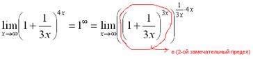
When the expression under the limit sign is in a degree, this is the first sign that you need to try to apply the second wonderful limit.

But first, as always, we try to substitute an infinitely large number into the expression, the principle by which this is done is discussed in the lesson Limits. Examples of solutions.

It is easy to notice that when the base of the degree is , and the exponent is , that is, there is uncertainty of the form:

This uncertainty is precisely revealed with the help of the second remarkable limit. But, as often happens, the second wonderful limit does not lie on a silver platter, and it needs to be artificially organized. You can reason as follows: in this example the parameter is , which means that we also need to organize in the indicator. To do this, we raise the base to the power, and so that the expression does not change, we raise it to the power:

When the task is completed by hand, we mark with a pencil:

Almost everything is ready, the terrible degree has turned into a nice letter:

In this case, we move the limit icon itself to the indicator: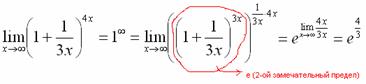

Example 7

Find the limit

Attention! This type of limit occurs very often, please study this example very carefully.

Let's try to substitute an infinitely large number into the expression under the limit sign:

The result is uncertainty. But the second remarkable limit applies to the uncertainty of the form. What to do? We need to convert the base of the degree. We reason like this: in the denominator we have , which means that in the numerator we also need to organize .

This online math calculator will help you if you need it calculate the limit of a function. Program solution limits not only gives the answer to the problem, it leads detailed solution with explanations, i.e. displays the limit calculation process.

This program can be useful for high school students in general education schools when preparing for tests and exams, when testing knowledge before the Unified State Exam, and for parents to control the solution of many problems in mathematics and algebra. Or maybe it’s too expensive for you to hire a tutor or buy new textbooks? Or do you just want to get your math or algebra homework done as quickly as possible? In this case, you can also use our programs with detailed solutions.

In this way, you can conduct your own training and/or training of your younger brothers or sisters, while the level of education in the field of solving problems increases.

It was discovered that some scripts necessary to solve this problem were not loaded, and the program may not work.
You may have AdBlock enabled.
In this case, disable it and refresh the page.

Because There are a lot of people willing to solve the problem, your request has been queued.
In a few seconds the solution will appear below.
Please wait sec...

If you noticed an error in the solution, then you can write about this in the Feedback Form.
Don't forget indicate which task you decide what enter in the fields.

Our games, puzzles, emulators:

A little theory.

Limit of the function at x->x 0

Let the function f(x) be defined on some set X and let the point \(x_0 \in X\) or \(x_0 \notin X\)

Let us take from X a sequence of points different from x 0:
x 1 , x 2 , x 3 , ..., x n , ... (1)
converging to x*. The function values ​​at the points of this sequence also form a numerical sequence
f(x 1), f(x 2), f(x 3), ..., f(x n), ... (2)
and one can raise the question of the existence of its limit.

Definition. The number A is called the limit of the function f(x) at the point x = x 0 (or at x -> x 0), if for any sequence (1) of values ​​of the argument x different from x 0 converging to x 0, the corresponding sequence (2) of values function converges to number A.

$$ \lim_(x\to x_0)( f(x)) = A $$

The function f(x) can have only one limit at the point x 0. This follows from the fact that the sequence
(f(x n)) has only one limit.

There is another definition of the limit of a function.

Definition The number A is called the limit of the function f(x) at the point x = x 0 if for any number \(\varepsilon > 0\) there is a number \(\delta > 0\) such that for all \(x \in X, \; x \neq x_0 \), satisfying the inequality \(|x-x_0| Using logical symbols, this definition can be written as
\((\forall \varepsilon > 0) (\exists \delta > 0) (\forall x \in X, \; x \neq x_0, \; |x-x_0| Note that the inequalities \(x \neq x_0 , \; |x-x_0| The first definition is based on the concept of the limit of a number sequence, so it is often called the “in the language of sequences” definition. The second definition is called the “in the language of \(\varepsilon - \delta \)”.
These two definitions of the limit of a function are equivalent and you can use either of them depending on which is more convenient for solving a particular problem.

Note that the definition of the limit of a function “in the language of sequences” is also called the definition of the limit of a function according to Heine, and the definition of the limit of a function “in the language \(\varepsilon - \delta \)” is also called the definition of the limit of a function according to Cauchy.

Limit of the function at x->x 0 - and at x->x 0 +

In what follows, we will use the concepts of one-sided limits of a function, which are defined as follows.

Definition The number A is called the right (left) limit of the function f(x) at the point x 0 if for any sequence (1) converging to x 0, the elements x n of which are greater (less than) x 0, the corresponding sequence (2) converges to A.

Symbolically it is written like this:
$$ \lim_(x \to x_0+) f(x) = A \; \left(\lim_(x \to x_0-) f(x) = A \right) $$

We can give an equivalent definition of one-sided limits of a function “in the language \(\varepsilon - \delta \)”:

Definition a number A is called the right (left) limit of the function f(x) at the point x 0 if for any \(\varepsilon > 0\) there exists \(\delta > 0\) such that for all x satisfying the inequalities \(x_0 Symbolic entries:

In this topic, we will analyze the formulas that can be obtained using the second remarkable limit (a topic dedicated directly to the second remarkable limit is located). Let me remind you of two formulations of the second remarkable limit that will be needed in this section: $\lim_(x\to\infty)\left(1+\frac(1)(x)\right)^x=e$ and $\lim_(x \to\ 0)\left(1+x\right)^\frac(1)(x)=e$.

Usually I present formulas without proof, but for this page, I think I’ll make an exception. The point is that the proof of the consequences of the second remarkable limit contains some techniques that are useful in directly solving problems. Well, generally speaking, it is advisable to know how this or that formula is proven. This allows us to better understand its internal structure, as well as the limits of applicability. But since the evidence may not be of interest to all readers, I will hide it under the notes located after each consequence.

Corollary #1

Evidence of corollary No. 1: show\hide

Since at $x\to 0$ we have $\ln(1+x)\to 0$, then in the limit under consideration there is an uncertainty of the form $\frac(0)(0)$. To reveal this uncertainty, let us present the expression $\frac(\ln(1+x))(x)$ in the following form: $\frac(1)(x)\cdot\ln(1+x)$. Now let's factor $\frac(1)(x)$ into the power of the expression $(1+x)$ and apply the second remarkable limit:

$$ \lim_(x\to\ 0) \frac(\ln(1+x))(x)=\left| \frac(0)(0) \right|= \lim_(x\to\ 0) \left(\frac(1)(x)\cdot\ln(1+x)\right)=\lim_(x\ to\ 0)\ln(1+x)^(\frac(1)(x))=\ln e=1. $$

Once again we have uncertainty of the form $\frac(0)(0)$. We will rely on the formula we have already proven. Since $\log_a t=\frac(\ln t)(\ln a)$, then $\log_a (1+x)=\frac(\ln(1+x))(\ln a)$.

$$ \lim_(x\to\ 0) \frac(\log_a (1+x))(x)=\left| \frac(0)(0) \right|=\lim_(x\to\ 0)\frac(\ln(1+x))( x \ln a)=\frac(1)(\ln a)\ lim_(x\to\ 0)\frac(\ln(1+x))( x)=\frac(1)(\ln a)\cdot 1=\frac(1)(\ln a). $$

Corollary #2

Evidence of corollary No. 2: show/hide

Since at $x\to 0$ we have $e^x-1\to 0$, then in the limit under consideration there is an uncertainty of the form $\frac(0)(0)$. To reveal this uncertainty, let us change the variable, denoting $t=e^x-1$. Since $x\to 0$, then $t\to 0$. Next, from the formula $t=e^x-1$ we get: $e^x=1+t$, $x=\ln(1+t)$.

$$ \lim_(x\to\ 0) \frac(e^x-1)(x)=\left| \frac(0)(0) \right|=\left | \begin(aligned) & t=e^x-1;\; t\to 0.\\ & x=\ln(1+t).\end (aligned) \right|= \lim_(t\to 0)\frac(t)(\ln(1+t))= \lim_(t\to 0)\frac(1)(\frac(\ln(1+t))(t))=\frac(1)(1)=1. $$

Once again we have uncertainty of the form $\frac(0)(0)$. We will rely on the formula we have already proven. Since $a^x=e^(x\ln a)$, then:

$$ \lim_(x\to\ 0) \frac(a^(x)-1)(x)=\left| \frac(0)(0) \right|=\lim_(x\to 0)\frac(e^(x\ln a)-1)(x)=\ln a\cdot \lim_(x\to 0 )\frac(e^(x\ln a)-1)(x \ln a)=\ln a \cdot 1=\ln a. $$

Corollary #3

Evidence of corollary No. 3: show\hide

Once again we are dealing with uncertainty of the form $\frac(0)(0)$. Since $(1+x)^\alpha=e^(\alpha\ln(1+x))$, we get:

$$ \lim_(x\to\ 0) \frac((1+x)^\alpha-1)(x)= \left| \frac(0)(0) \right|= \lim_(x\to\ 0)\frac(e^(\alpha\ln(1+x))-1)(x)= \lim_(x\to \ 0)\left(\frac(e^(\alpha\ln(1+x))-1)(\alpha\ln(1+x))\cdot \frac(\alpha\ln(1+x) )(x) \right)=\\ =\alpha\lim_(x\to\ 0) \frac(e^(\alpha\ln(1+x))-1)(\alpha\ln(1+x ))\cdot \lim_(x\to\ 0)\frac(\ln(1+x))(x)=\alpha\cdot 1\cdot 1=\alpha. $$

Example No. 1

Calculate the limit $\lim_(x\to\ 0) \frac(e^(9x)-1)(\sin 5x)$.

We have an uncertainty of the form $\frac(0)(0)$. To reveal this uncertainty, we will use the formula. To fit our limit to this formula, we should keep in mind that the expressions in the power of $e$ and in the denominator must coincide. In other words, there is no place for sine in the denominator. The denominator should be $9x$. Additionally, the solution to this example will use the first remarkable limit.

$$ \lim_(x\to\ 0) \frac(e^(9x)-1)(\sin 5x)=\left|\frac(0)(0) \right|=\lim_(x\to\ 0) \left(\frac(e^(9x)-1)(9x)\cdot\frac(9x)(\sin 5x) \right) =\frac(9)(5)\cdot\lim_(x\ to\ 0) \left(\frac(e^(9x)-1)(9x)\cdot\frac(1)(\frac(\sin 5x)(5x)) \right)=\frac(9)( 5)\cdot 1 \cdot 1=\frac(9)(5). $$

Answer: $\lim_(x\to\ 0) \frac(e^(9x)-1)(\sin 5x)=\frac(9)(5)$.

Example No. 2

Calculate the limit $\lim_(x\to\ 0) \frac(\ln\cos x)(x^2)$.

We have an uncertainty of the form $\frac(0)(0)$ (let me remind you that $\ln\cos 0=\ln 1=0$). To reveal this uncertainty, we will use the formula. First, let's take into account that $\cos x=1-2\sin^2 \frac(x)(2)$ (see printout on trigonometric functions). Now $\ln\cos x=\ln\left(1-2\sin^2 \frac(x)(2)\right)$, so in the denominator we should get the expression $-2\sin^2 \frac(x )(2)$ (to fit our example to the formula). In the further solution, the first remarkable limit will be used.

$$ \lim_(x\to\ 0) \frac(\ln\cos x)(x^2)=\left| \frac(0)(0) \right|=\lim_(x\to\ 0) \frac(\ln\left(1-2\sin^2 \frac(x)(2)\right))(x ^2)= \lim_(x\to\ 0) \left(\frac(\ln\left(1-2\sin^2 \frac(x)(2)\right))(-2\sin^2 \frac(x)(2))\cdot\frac(-2\sin^2 \frac(x)(2))(x^2) \right)=\\ =-\frac(1)(2) \lim_(x\to\ 0) \left(\frac(\ln\left(1-2\sin^2 \frac(x)(2)\right))(-2\sin^2 \frac(x )(2))\cdot\left(\frac(\sin\frac(x)(2))(\frac(x)(2))\right)^2 \right)=-\frac(1)( 2)\cdot 1\cdot 1^2=-\frac(1)(2). $$

Answer: $\lim_(x\to\ 0) \frac(\ln\cos x)(x^2)=-\frac(1)(2)$.

There are several remarkable limits, but the most famous are the first and second remarkable limits. The remarkable thing about these limits is that they are widely used and with their help you can find other limits found in numerous problems. This is what we will do in the practical part of this lesson. To solve problems by reducing them to the first or second remarkable limit, there is no need to reveal the uncertainties contained in them, since the values ​​of these limits have long been deduced by great mathematicians.

The first wonderful limit is called the limit of the ratio of the sine of an infinitesimal arc to the same arc, expressed in radian measure:

Let's move on to solving problems at the first remarkable limit. Note: if there is a trigonometric function under the limit sign, this is an almost sure sign that this expression can be reduced to the first remarkable limit.

Example 1. Find the limit.

Solution. Substitution instead x zero leads to uncertainty:

.

The denominator is sine, therefore, the expression can be brought to the first remarkable limit. Let's start the transformation:

.

The denominator is the sine of three X, but the numerator has only one X, which means you need to get three X in the numerator. For what? To introduce 3 x = a and get the expression .

And we come to a variation of the first remarkable limit:

because it doesn’t matter which letter (variable) in this formula stands instead of X.

We multiply X by three and immediately divide:

.

In accordance with the first remarkable limit noticed, we replace the fractional expression:

Now we can finally solve this limit:

.

Example 2. Find the limit.

Solution. Direct substitution again leads to the “zero divided by zero” uncertainty:

.

To get the first remarkable limit, it is necessary that the x under the sine sign in the numerator and just the x in the denominator have the same coefficient. Let this coefficient be equal to 2. To do this, imagine the current coefficient for x as below, performing operations with fractions, we obtain:

.

Example 3. Find the limit.

Solution. When substituting, we again get the uncertainty “zero divided by zero”:

.

You probably already understand that from the original expression you can get the first wonderful limit multiplied by the first wonderful limit. To do this, we decompose the squares of the x in the numerator and the sine in the denominator into identical factors, and in order to get the same coefficients for the x and sine, we divide the x in the numerator by 3 and immediately multiply by 3. We get:

.

Example 4. Find the limit.

Solution. Once again we get the uncertainty “zero divided by zero”:

.

We can obtain the ratio of the first two remarkable limits. We divide both the numerator and the denominator by x. Then, so that the coefficients for sines and xes coincide, we multiply the upper x by 2 and immediately divide by 2, and multiply the lower x by 3 and immediately divide by 3. We get:

Example 5. Find the limit.

Solution. And again the uncertainty of “zero divided by zero”:

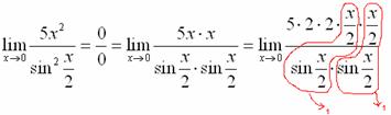
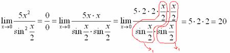
We remember from trigonometry that tangent is the ratio of sine to cosine, and the cosine of zero is equal to one. We carry out the transformations and get:

.

Example 6. Find the limit.

Solution. The trigonometric function under the sign of a limit again suggests the use of the first remarkable limit. We represent it as the ratio of sine to cosine.