The confidence interval shows. Test the capabilities of paid solutions

"Katren-Style" continues the publication of Konstantin Kravchik's series on medical statistics. In two previous articles, the author dealt with the explanation of concepts such as and.

Konstantin Kravchik

Mathematician-analyst. Specialist in statistical research in medicine and humanities

City: Moscow

Very often in articles on clinical studies you can find a mysterious phrase: “confidence interval” (95 % CI or 95 % CI - confidence interval). For example, an article might write: “To assess the significance of differences, the Student’s t-test was used to calculate the 95 % confidence interval.”

What is the value of the “95 % confidence interval” and why calculate it?

What is a confidence interval? - This is the range within which the true population means lie. Are there “untrue” averages? In a sense, yes, they do. In we explained that it is impossible to measure the parameter of interest in the entire population, so researchers are content with a limited sample. In this sample (for example, by body weight) there is one average value (a certain weight), by which we judge the average value in the entire population. However, it is unlikely that the average weight in a sample (especially a small one) will coincide with the average weight in the general population. Therefore, it is more correct to calculate and use the range of population averages.

For example, imagine that the 95% confidence interval (95% CI) for hemoglobin is 110 to 122 g/L. This means that there is a 95% chance that the true mean hemoglobin value in the population will be between 110 and 122 g/L. In other words, we do not know the average hemoglobin value in the population, but we can, with 95 % probability, indicate a range of values ​​for this trait.

Confidence intervals are particularly relevant for differences in means between groups, or effect sizes as they are called.

Let's say we compared the effectiveness of two iron preparations: one that has been on the market for a long time and one that has just been registered. After the course of therapy, we assessed the hemoglobin concentration in the studied groups of patients, and the statistical program calculated that the difference between the average values ​​of the two groups was, with a 95 % probability, in the range from 1.72 to 14.36 g/l (Table 1).

Table 1. Test for independent samples
(groups are compared by hemoglobin level)

This should be interpreted as follows: in some patients in the general population who take a new drug, hemoglobin will be higher on average by 1.72–14.36 g/l than in those who took an already known drug.

In other words, in the general population, the difference in average hemoglobin values ​​between groups is within these limits with a 95% probability. It will be up to the researcher to judge whether this is a lot or a little. The point of all this is that we are not working with one average value, but with a range of values, therefore, we more reliably estimate the difference in a parameter between groups.

In statistical packages, at the discretion of the researcher, you can independently narrow or expand the boundaries of the confidence interval. By lowering the confidence interval probabilities, we narrow the range of means. For example, at 90 % CI the range of means (or difference in means) will be narrower than at 95 %.

Conversely, increasing the probability to 99 % expands the range of values. When comparing groups, the lower limit of the CI may cross the zero mark. For example, if we expanded the boundaries of the confidence interval to 99 %, then the boundaries of the interval ranged from –1 to 16 g/l. This means that in the general population there are groups, the difference in means between which for the characteristic being studied is equal to 0 (M = 0).

Using a confidence interval, you can test statistical hypotheses. If the confidence interval crosses the zero value, then the null hypothesis, which assumes that the groups do not differ on the parameter being studied, is true. The example is described above where we expanded the boundaries to 99 %. Somewhere in the general population we found groups that did not differ in any way.

95% confidence interval of the difference in hemoglobin, (g/l)

The figure shows the 95% confidence interval for the difference in mean hemoglobin values ​​between the two groups. The line passes through the zero mark, therefore there is a difference between the means of zero, which confirms the null hypothesis that the groups do not differ. The range of difference between groups is from –2 to 5 g/L. This means that hemoglobin can either decrease by 2 g/L or increase by 5 g/L.

The confidence interval is a very important indicator. Thanks to it, you can see whether the differences in the groups were really due to the difference in means or due to a large sample, since with a large sample the chances of finding differences are greater than with a small one.

In practice it might look like this. We took a sample of 1000 people, measured hemoglobin levels and found that the confidence interval for the difference in means ranged from 1.2 to 1.5 g/l. The level of statistical significance in this case p

We see that the hemoglobin concentration increased, but almost imperceptibly, therefore, statistical significance appeared precisely due to the sample size.

Confidence intervals can be calculated not only for means, but also for proportions (and risk ratios). For example, we are interested in the confidence interval of the proportions of patients who achieved remission while taking a developed drug. Let us assume that the 95 % CI for the proportions, i.e., for the proportion of such patients, lies in the range of 0.60–0.80. Thus, we can say that our medicine has a therapeutic effect in 60 to 80 % of cases.

From this article you will learn:

What's happened confidence interval?

What's the point 3 sigma rules?

How can you apply this knowledge in practice?

Nowadays, due to an overabundance of information associated with a large assortment of products, sales directions, employees, areas of activity, etc., it can be difficult to highlight the main thing, which, first of all, is worth paying attention to and making efforts to manage. Definition confidence interval and analysis of actual values ​​going beyond its boundaries - a technique that will help you highlight situations, influencing changing trends. You will be able to develop positive factors and reduce the influence of negative ones. This technology is used in many well-known global companies.

There are so-called " alerts", which inform managers that the next value is in a certain direction went beyond confidence interval. What does this mean? This is a signal that some unusual event has occurred, which may change the existing trend in this direction. This is a signal to that to figure it out in the situation and understand what influenced it.

For example, consider several situations. We calculated the sales forecast with forecast limits for 100 product items for 2011 by month and actual sales in March:

1. For “Sunflower oil” they broke through the upper limit of the forecast and did not fall into the confidence interval.
2. For “Dry yeast” we exceeded the lower limit of the forecast.
3. “Oatmeal Porridge” has broken through the upper limit.

For other products, actual sales were within the given forecast limits. Those. their sales were within expectations. So, we identified 3 products that went beyond the borders and began to figure out what influenced them to go beyond the borders:

1. For Sunflower Oil, we entered a new distribution network, which gave us additional sales volume, which led to us going beyond the upper limit. For this product, it is worth recalculating the forecast until the end of the year, taking into account the sales forecast for this network.
2. For “Dry Yeast”, the car got stuck at customs, and there was a shortage within 5 days, which affected the decline in sales and exceeded the lower limit. It may be worthwhile to figure out what caused it and try not to repeat this situation.
3. A sales promotion event was launched for Oatmeal Porridge, which gave a significant increase in sales and led to the company going beyond the forecast.

We identified 3 factors that influenced the going beyond the forecast limits. There can be much more of them in life. To increase the accuracy of forecasting and planning, factors that lead to the fact that actual sales may go beyond the forecast, it is worth highlighting and building forecasts and plans for them separately. And then consider their impact on the main sales forecast. You can also regularly assess the impact of these factors and change the situation for the better. by reducing the influence of negative and increasing the influence of positive factors.

With a confidence interval we can:

1. Select directions, which are worth paying attention to, because events have occurred in these directions that may affect change in trend.
2. Identify factors, which really influence the change in the situation.
3. Accept informed decision(for example, about purchasing, planning, etc.).

Now let's look at what a confidence interval is and how to calculate it in Excel using an example.

What is a confidence interval?

Confidence interval is the forecast boundaries (upper and lower), within which with a given probability (sigma) actual values ​​will appear.

Those. We calculate the forecast - this is our main guideline, but we understand that the actual values ​​are unlikely to be 100% equal to our forecast. And the question arises, within what boundaries actual values ​​may fall, if the current trend continues? And this question will help us answer confidence interval calculation, i.e. - upper and lower limits of the forecast.

What is a given probability sigma?

When calculating confidence interval we can set probability hits actual values within the given forecast limits. How to do this? To do this, we set the value of sigma and, if sigma is equal to:

3 sigma- then, the probability of the next actual value falling into the confidence interval will be 99.7%, or 300 to 1, or there is a 0.3% probability of going beyond the boundaries.

2 sigma- then, the probability of the next value falling within the boundaries is ≈ 95.5%, i.e. the odds are about 20 to 1, or there is a 4.5% chance of going overboard.

1 sigma- then the probability is ≈ 68.3%, i.e. the odds are approximately 2 to 1, or there is a 31.7% chance that the next value will fall outside the confidence interval.

We formulated 3 sigma rule,which says that hit probability another random value into the confidence interval with a given value three sigma is 99.7%.

The great Russian mathematician Chebyshev proved the theorem that there is a 10% probability of going beyond the forecast limits with a given value of three sigma. Those. the probability of falling within the 3-sigma confidence interval will be at least 90%, while an attempt to calculate the forecast and its boundaries “by eye” is fraught with much more significant errors.

How to calculate a confidence interval yourself in Excel?

Let's look at the calculation of the confidence interval in Excel (i.e., the upper and lower limits of the forecast) using an example. We have a time series - sales by month for 5 years. See attached file.

To calculate the forecast limits, we calculate:

1. Sales forecast().
2. Sigma - standard deviation forecast models from actual values.
3. Three sigma.
4. Confidence interval.

1. Sales forecast.

=(RC[-14] (time series data)- RC[-1] (model value))^2(squared)

3. For each month, let’s sum up the deviation values ​​from stage 8 Sum((Xi-Ximod)^2), i.e. Let's sum up January, February... for each year.

To do this, use the formula =SUMIF()

SUMIF(array with period numbers inside the cycle (for months from 1 to 12); link to the period number in the cycle; link to an array with squares of the difference between the source data and period values)

4. Calculate the standard deviation for each period in the cycle from 1 to 12 (stage 10 in the attached file).

To do this, we extract the root from the value calculated at stage 9 and divide by the number of periods in this cycle minus 1 = SQRT((Sum(Xi-Ximod)^2/(n-1))

Let's use the formulas in Excel =ROOT(R8 (link to (Sum(Xi-Ximod)^2)/(COUNTIF($O$8:$O$67 (link to array with cycle numbers); O8 (link to a specific cycle number that we count in the array))-1))

Using the Excel formula = COUNTIF we count the number n

Having calculated the standard deviation of the actual data from the forecast model, we obtained the sigma value for each month - stage 10 in the attached file.

3. Let's calculate 3 sigma.

At stage 11 we set the number of sigmas - in our example “3” (stage 11 in the attached file):

Also convenient for practice sigma values:

1.64 sigma - 10% chance of exceeding the limit (1 chance in 10);

1.96 sigma - 5% chance of going beyond limits (1 chance in 20);

2.6 sigma - 1% chance of exceeding limits (1 chance in 100).

5) Calculating three sigma, for this we multiply the “sigma” values ​​for each month by “3”.

3. Determine the confidence interval.

1. Upper forecast limit- sales forecast taking into account growth and seasonality + (plus) 3 sigma;
2. Lower forecast limit- sales forecast taking into account growth and seasonality – (minus) 3 sigma;

For the convenience of calculating the confidence interval for a long period (see attached file), we will use the Excel formula =Y8+VLOOKUP(W8,$U$8:$V$19,2,0), Where

Y8- sales forecast;

W8- the number of the month for which we will take the 3-sigma value;

Those. Upper forecast limit= “sales forecast” + “3 sigma” (in the example, VLOOKUP(month number; table with 3 sigma values; column from which we extract the sigma value equal to the month number in the corresponding row; 0)).

Lower forecast limit= “sales forecast” minus “3 sigma”.

So, we calculated the confidence interval in Excel.

Now we have a forecast and a range with boundaries within which the actual values ​​will fall with a given sigma probability.

In this article, we looked at what sigma and the three-sigma rule are, how to determine a confidence interval, and why you can use this technique in practice.

We wish you accurate forecasts and success!

How Forecast4AC PRO can help youwhen calculating the confidence interval?:

Forecast4AC PRO will automatically calculate the upper or lower bounds of the forecast for more than 1000 time series simultaneously;

The ability to analyze the boundaries of the forecast in comparison with the forecast, trend and actual sales on the chart with one keystroke;

In the Forcast4AC PRO program it is possible to set the sigma value from 1 to 3.

Join us!

Download free forecasting and business analysis apps:

• Novo Forecast Lite- automatic forecast calculation V Excel.
• 4analytics - ABC-XYZ analysis and emissions analysis Excel.
• Qlik Sense Desktop and QlikViewPersonal Edition - BI systems for data analysis and visualization.

Test the capabilities of paid solutions:

• Novo Forecast PRO- forecasting in Excel for large data sets.

Confidence interval(CI; in English, confidence interval - CI) obtained in a study with a sample gives a measure of the accuracy (or uncertainty) of the study results in order to draw conclusions about the population of all such patients (the general population). The correct definition of a 95% CI can be formulated as follows: 95% of such intervals will contain the true value in the population. This interpretation is somewhat less accurate: CI is the range of values ​​within which you can be 95% sure that it contains the true value. When using a CI, the emphasis is on determining the quantitative effect, as opposed to the P value, which is obtained by testing statistical significance. The P value does not estimate any quantity, but rather serves as a measure of the strength of evidence against the null hypothesis of “no effect.” The value of P by itself does not tell us anything about the magnitude of the difference, or even about its direction. Therefore, independent P values ​​are absolutely uninformative in articles or abstracts. In contrast, the CI indicates both the size of the effect of immediate interest, such as the benefit of a treatment, and the strength of the evidence. Therefore, DI is directly related to the practice of EBM.

The estimation approach to statistical analysis, exemplified by CI, aims to measure the quantity of an effect of interest (sensitivity of a diagnostic test, rate of predicted cases, relative risk reduction with treatment, etc.) and also to measure the uncertainty in that effect. Most often, the CI is the range of values ​​on either side of the estimate in which the true value is likely to lie, and you can be 95% sure of it. The agreement to use the 95% probability is arbitrary, as is the P value.<0,05 для оценки статистической значимости, и авторы иногда используют 90% или 99% ДИ. Заметим, что слово «интервал» означает диапазон величин и поэтому стоит в единственном числе. Две величины, которые ограничивают интервал, называются «доверительными пределами».

CI is based on the idea that the same study performed on different samples of patients would not produce identical results, but that their results would be distributed around a true but unknown value. In other words, CI describes it as “sample-dependent variability.” The CI does not reflect additional uncertainty due to other reasons; in particular, it does not include the impact of selective loss to follow-up, poor compliance or inaccurate outcome measurement, lack of blinding, etc. The CI therefore always underestimates the total amount of uncertainty.

Confidence Interval Calculation

Table A1.1. Standard errors and confidence intervals for selected clinical measurements

Typically, a CI is calculated from an observed estimate of a quantity, such as the difference (d) between two proportions, and the standard error (SE) in the estimate of that difference. The approximate 95% CI obtained in this way is d ± 1.96 SE. The formula changes according to the nature of the outcome measure and the scope of the CI. For example, in a randomized, placebo-controlled trial of an acellular pertussis vaccine, 72 of 1670 (4.3%) infants who received the vaccine developed pertussis and 240 of 1665 (14.4%) in the control group. The percentage difference, known as the absolute risk reduction, is 10.1%. The SE of this difference is 0.99%. Accordingly, the 95% CI is 10.1% + 1.96 x 0.99%, i.e. from 8.2 to 12.0.

Despite their different philosophical approaches, CIs and statistical significance tests are closely related mathematically.

Thus, the P value is “significant”, i.e. R<0,05 соответствует 95% ДИ, который исключает величину эффекта, указывающую на отсутствие различия. Например, для различия между двумя средними пропорциями это ноль, а для относительного риска или отношения шансов - единица. При некоторых обстоятельствах эти два подхода могут быть не совсем эквивалентны. Преобладающая точка зрения: оценка с помощью ДИ - предпочтительный подход к суммированию результатов исследования, но ДИ и величина Р взаимодополняющи, и во многих статьях используются оба способа представления результатов.

The uncertainty (inaccuracy) of the estimate, expressed in CI, is largely related to the square root of the sample size. Small samples provide less information than large ones, and the CI is correspondingly wider in a smaller sample. For example, an article comparing the performance of three tests used to diagnose Helicobacter pylori infection reported a sensitivity of the urea breath test of 95.8% (95% CI 75–100). While the 95.8% figure is impressive, the small sample of 24 adult patients with J. pylori means that there is significant uncertainty in this estimate, as shown by the wide CI. Indeed, the lower limit of 75% is much lower than the 95.8% estimate. If the same sensitivity were observed in a sample of 240 people, the 95% CI would be 92.5–98.0, giving more assurance that the test is highly sensitive.

In randomized controlled trials (RCTs), nonsignificant results (i.e., those with P >0.05) are particularly susceptible to misinterpretation. The CI is particularly useful here because it shows how consistent the results are with the clinically useful true effect. For example, in an RCT comparing colonic suture and staple anastomosis, wound infection developed in 10.9% and 13.5% of patients, respectively (P = 0.30). The 95% CI for this difference is 2.6% (−2 to +8). Even in this study of 652 patients, it remains possible that there is a modest difference in the incidence of infections resulting from the two procedures. The less research, the greater the uncertainty. Sung et al. performed an RCT to compare octreotide infusion with acute sclerotherapy for acute variceal bleeding in 100 patients. In the octreotide group, the bleeding control rate was 84%; in the sclerotherapy group - 90%, which gives P = 0.56. Note that rates of ongoing bleeding are similar to those for wound infection in the study mentioned. In this case, however, the 95% CI for the difference between interventions is 6% (−7 to +19). This range is quite wide compared to the 5% difference that would be of clinical interest. Clearly, the study does not rule out a significant difference in effectiveness. Therefore, the authors’ conclusion “octreotide infusion and sclerotherapy are equally effective in the treatment of bleeding from varicose veins” is definitely invalid. In cases like this, where, as here, the 95% CI for absolute risk reduction (ARR) includes zero, the CI for NNT (number needed to treat) is quite difficult to interpret . The NPL and its CI are obtained from the reciprocals of the ACP (multiplying by 100 if these values ​​are given as percentages). Here we get NPL = 100: 6 = 16.6 with a 95% CI of -14.3 to 5.3. As can be seen from footnote “d” in table. A1.1, this CI includes values ​​of NPL from 5.3 to infinity and NPL from 14.3 to infinity.

CIs can be constructed for most commonly used statistical estimates or comparisons. For RCTs, it includes the difference between mean proportions, relative risks, odds ratios, and NLRs. Similarly, CIs can be obtained for all the major estimates made in diagnostic test accuracy studies—sensitivity, specificity, positive predictive value (all of which are simple proportions), and likelihood ratios—estimates obtained in meta-analyses and comparison-with-control studies. A personal computer program that covers many of these uses of MDIs is available with the second edition of Statistics with Confidence. Macros for calculating CIs for proportions are available free of charge for Excel and the statistical programs SPSS and Minitab at http://www.uwcm.ac.uk/study/medicine/epidemiology_statistics/research/statistics/proportions, htm.

Multiple estimates of treatment effect

While constructing CIs is desirable for primary study outcomes, they are not necessary for all outcomes. The CI concerns clinically important comparisons. For example, when comparing two groups, the correct CI is the one constructed for the difference between groups, as shown in the examples above, and not the CI that can be constructed for the estimate in each group. Not only is it not helpful to provide separate CIs for estimates in each group, this presentation can be misleading. Likewise, the correct approach when comparing the effectiveness of treatments in different subgroups is to compare two (or more) subgroups directly. It is incorrect to assume that a treatment is effective in only one subgroup if its CI excludes the value corresponding to no effect and the others do not. CIs are also useful when comparing results across multiple subgroups. In Fig. A 1.1 shows the relative risk of eclampsia in women with preeclampsia in subgroups of women from a placebo-controlled RCT of magnesium sulfate.

Rice. A1.2. The forest plot shows the results of 11 randomized clinical trials of bovine rotavirus vaccine for the prevention of diarrhea compared with placebo. A 95% confidence interval was used to estimate the relative risk of diarrhea. The size of the black square is proportional to the amount of information. In addition, the summary estimate of treatment effectiveness and the 95% confidence interval (indicated by a diamond) are shown. The meta-analysis used a random effects model larger than some pre-specified ones; for example, this could be the size used in calculating the sample size. A more stringent criterion requires that the entire CI range show benefit greater than a prespecified minimum.

We have already discussed the fallacy of taking a lack of statistical significance as an indication that two treatments are equally effective. It is equally important not to equate statistical significance with clinical importance. Clinical importance can be assumed when the result is statistically significant and the magnitude of the estimate of treatment effectiveness

Studies can show whether results are statistically significant and which are clinically important and which are not. In Fig. A1.2 shows the results of four tests, for which the entire CI<1, т.е. их результаты статистически значимы при Р <0,05 , . После высказанного предположения о том, что клинически важным различием было бы сокращение риска диареи на 20% (ОР = 0,8), все эти испытания показали клинически значимую оценку сокращения риска, и лишь в исследовании Treanor весь 95% ДИ меньше этой величины. Два других РКИ показали клинически важные результаты, которые не были статистически значимыми. Обратите внимание, что в трёх испытаниях точечные оценки эффективности лечения были почти идентичны, но ширина ДИ различалась (отражает размер выборки). Таким образом, по отдельности доказательная сила этих РКИ различна.

There are two types of estimates in statistics: point and interval. Point estimate is a single sample statistic that is used to estimate a population parameter. For example, the sample mean is a point estimate of the mathematical expectation of the population, and the sample variance S 2- point estimate of population variance σ 2. it has been shown that the sample mean is an unbiased estimate of the mathematical expectation of the population. A sample mean is called unbiased because the average of all sample means (with the same sample size) n) is equal to the mathematical expectation of the general population.

In order for the sample variance S 2 became an unbiased estimate of the population variance σ 2, the denominator of the sample variance should be set equal to n – 1 , not n. In other words, the population variance is the average of all possible sample variances.

When estimating population parameters, it should be kept in mind that sample statistics such as , depend on specific samples. To take this fact into account, to obtain interval estimation mathematical expectation of the general population, analyze the distribution of sample means (for more details, see). The constructed interval is characterized by a certain confidence level, which represents the probability that the true population parameter is estimated correctly. Similar confidence intervals can be used to estimate the proportion of a characteristic r and the main distributed mass of the population.

Download the note in or format, examples in format

Constructing a confidence interval for the mathematical expectation of the population with a known standard deviation

Constructing a confidence interval for the share of a characteristic in the population

This section extends the concept of confidence interval to categorical data. This allows us to estimate the share of the characteristic in the population r using sample share rS= X/n. As indicated, if the quantities nr And n(1 – p) exceed the number 5, the binomial distribution can be approximated as normal. Therefore, to estimate the share of a characteristic in the population r it is possible to construct an interval whose confidence level is equal to (1 – α)х100%.

Where pS- sample proportion of the characteristic equal to X/n, i.e. number of successes divided by sample size, r- the share of the characteristic in the general population, Z- critical value of the standardized normal distribution, n- sample size.

Example 3. Let's assume that a sample consisting of 100 invoices filled out during the last month is extracted from the information system. Let's say that 10 of these invoices were compiled with errors. Thus, r= 10/100 = 0.1. The 95% confidence level corresponds to the critical value Z = 1.96.

Thus, the probability that between 4.12% and 15.88% of invoices contain errors is 95%.

For a given sample size, the confidence interval containing the proportion of the trait in the population appears wider than for a continuous random variable. This is because measurements of a continuous random variable contain more information than measurements of categorical data. In other words, categorical data that takes only two values ​​contains insufficient information to estimate the parameters of their distribution.

INcalculating estimates extracted from a finite population

Estimation of mathematical expectation. Correction factor for the final population ( fpc) was used to reduce the standard error by a factor. When calculating confidence intervals for population parameter estimates, a correction factor is applied in situations where samples are drawn without being returned. Thus, a confidence interval for the mathematical expectation having a confidence level equal to (1 – α)х100%, is calculated by the formula:

Example 4. To illustrate the use of the correction factor for a finite population, let us return to the problem of calculating the confidence interval for the average amount of invoices, discussed above in Example 3. Suppose that a company issues 5,000 invoices per month, and X̅=110.27 dollars, S= $28.95, N = 5000, n = 100, α = 0.05, t 99 = 1.9842. Using formula (6) we obtain:

Estimation of the share of a feature. When choosing without return, the confidence interval for the proportion of the attribute having a confidence level equal to (1 – α)х100%, is calculated by the formula:

Confidence Intervals and Ethical Issues

When sampling a population and drawing statistical conclusions, ethical issues often arise. The main one is how confidence intervals and point estimates of sample statistics agree. Publishing point estimates without specifying the associated confidence intervals (usually at the 95% confidence level) and the sample size from which they are derived can create confusion. This may give the user the impression that the point estimate is exactly what he needs to predict the properties of the entire population. Thus, it is necessary to understand that in any research the focus should be not on point estimates, but on interval estimates. In addition, special attention should be paid to the correct selection of sample sizes.

Most often, the objects of statistical manipulation are the results of sociological surveys of the population on certain political issues. At the same time, the survey results are published on the front pages of newspapers, and the sampling error and statistical analysis methodology are published somewhere in the middle. To prove the validity of the obtained point estimates, it is necessary to indicate the sample size on the basis of which they were obtained, the boundaries of the confidence interval and its level of significance.

Next note

Materials from the book Levin et al. Statistics for Managers are used. – M.: Williams, 2004. – p. 448–462

Central limit theorem states that with a sufficiently large sample size, the sample distribution of means can be approximated by a normal distribution. This property does not depend on the type of distribution of the population.

Target– teach students algorithms for calculating confidence intervals of statistical parameters.

When statistically processing data, the calculated arithmetic mean, coefficient of variation, correlation coefficient, difference criteria and other point statistics should receive quantitative confidence limits, which indicate possible fluctuations of the indicator in smaller and larger directions within the confidence interval.

Example 3.1 . The distribution of calcium in the blood serum of monkeys, as previously established, is characterized by the following sample indicators: = 11.94 mg%; = 0.127 mg%; n= 100. It is required to determine the confidence interval for the general average ( ) with confidence probability P = 0,95.

The general average is located with a certain probability in the interval:

, Where – sample arithmetic mean; t– Student’s test; – error of the arithmetic mean.

Using the table “Student’s t-test values” we find the value with a confidence probability of 0.95 and the number of degrees of freedom k= 100-1 = 99. It is equal to 1.982. Together with the values ​​of the arithmetic mean and statistical error, we substitute it into the formula:

or 11.69
12,19

Thus, with a probability of 95%, it can be stated that the general average of this normal distribution is between 11.69 and 12.19 mg%.

Example 3.2 . Determine the boundaries of the 95% confidence interval for the general variance ( ) distribution of calcium in the blood of monkeys, if it is known that
= 1.60, at n = 100.

To solve the problem you can use the following formula:

Where – statistical error of dispersion.

We find the sampling variance error using the formula:
. It is equal to 0.11. Meaning t- criterion with a confidence probability of 0.95 and the number of degrees of freedom k= 100–1 = 99 is known from the previous example.

Let's use the formula and get:

or 1.38
1,82

More accurately, the confidence interval of the general variance can be constructed using (chi-square) - Pearson test. The critical points for this criterion are given in a special table. When using the criterion To construct a confidence interval, a two-sided significance level is used. For the lower limit, the significance level is calculated using the formula
, for the top –
. For example, for the confidence level = 0,99= 0,010,= 0.990. Accordingly, according to the table of distribution of critical values , with calculated confidence levels and number of degrees of freedom k= 100 – 1= 99, find the values
And
. We get
equals 135.80, and
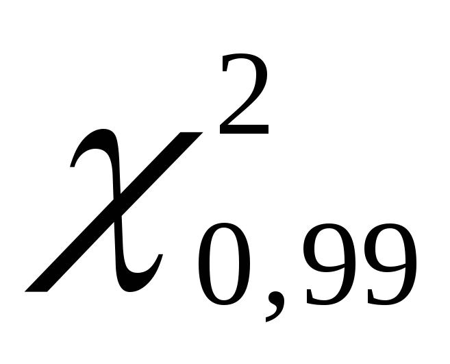equals 70.06.

To find confidence limits for the general variance using Let's use the formulas: for the lower boundary
, for the upper bound
. Let's substitute the found values ​​for the problem data into formulas:
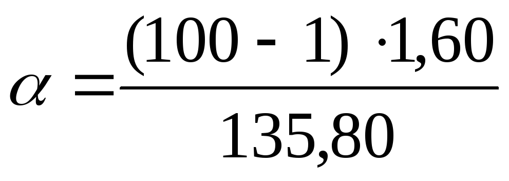= 1,17;
= 2.26. Thus, with a confidence probability P= 0.99 or 99% general variance will lie in the range from 1.17 to 2.26 mg% inclusive.

Example 3.3 . Among 1000 wheat seeds from the batch received at the elevator, 120 seeds were found infected with ergot. It is necessary to determine the probable boundaries of the general proportion of infected seeds in a given batch of wheat.

It is advisable to determine the confidence limits for the general share for all its possible values ​​using the formula:

,

Where n – number of observations; m– absolute size of one of the groups; t– normalized deviation.

The sample proportion of infected seeds is
or 12%. With confidence probability R= 95% normalized deviation ( t-Student's test at k =
)t = 1,960.

We substitute the available data into the formula:

Hence the boundaries of the confidence interval are equal to = 0.122–0.041 = 0.081, or 8.1%; = 0.122 + 0.041 = 0.163, or 16.3%.

Thus, with a confidence probability of 95% it can be stated that the general proportion of infected seeds is between 8.1 and 16.3%.

Example 3.4 . The coefficient of variation characterizing the variation of calcium (mg%) in the blood serum of monkeys was equal to 10.6%. Sample size n= 100. It is necessary to determine the boundaries of the 95% confidence interval for the general parameter Cv.

Limits of the confidence interval for the general coefficient of variation Cv are determined by the following formulas:

And
, Where K intermediate value calculated by the formula
.

Knowing that with confidence probability R= 95% normalized deviation (Student's test at k =
)t = 1.960, let’s first calculate the value TO:

.

or 9.3%

or 12.3%

Thus, the general coefficient of variation with a 95% confidence level lies in the range from 9.3 to 12.3%. With repeated samples, the coefficient of variation will not exceed 12.3% and will not be below 9.3% in 95 cases out of 100.

Questions for self-control:

Problems for independent solution.

1. The average percentage of fat in milk during lactation of Kholmogory crossbred cows was as follows: 3.4; 3.6; 3.2; 3.1; 2.9; 3.7; 3.2; 3.6; 4.0; 3.4; 4.1; 3.8; 3.4; 4.0; 3.3; 3.7; 3.5; 3.6; 3.4; 3.8. Establish confidence intervals for the general mean at 95% confidence level (20 points).

2. On 400 hybrid rye plants, the first flowers appeared on average 70.5 days after sowing. The standard deviation was 6.9 days. Determine the error of the mean and confidence intervals for the general mean and variance at the significance level W= 0.05 and W= 0.01 (25 points).

3. When studying the length of leaves of 502 specimens of garden strawberries, the following data were obtained: = 7.86 cm; σ = 1.32 cm, =± 0.06 cm. Determine confidence intervals for the arithmetic population mean with significance levels of 0.01; 0.02; 0.05. (25 points).

4. In a study of 150 adult men, the average height was 167 cm, and σ = 6 cm. What are the limits of the general mean and general variance with a confidence probability of 0.99 and 0.95? (25 points).

5. The distribution of calcium in the blood serum of monkeys is characterized by the following selective indicators: = 11.94 mg%, σ = 1,27, n = 100. Construct a 95% confidence interval for the general mean of this distribution. Calculate the coefficient of variation (25 points).

6. The total nitrogen content in the blood plasma of albino rats at the age of 37 and 180 days was studied. The results are expressed in grams per 100 cm 3 of plasma. At the age of 37 days, 9 rats had: 0.98; 0.83; 0.99; 0.86; 0.90; 0.81; 0.94; 0.92; 0.87. At the age of 180 days, 8 rats had: 1.20; 1.18; 1.33; 1.21; 1.20; 1.07; 1.13; 1.12. Set confidence intervals for the difference at a confidence level of 0.95 (50 points).

7. Determine the boundaries of the 95% confidence interval for the general variance of the distribution of calcium (mg%) in the blood serum of monkeys, if for this distribution the sample size is n = 100, statistical error of the sample variance s σ 2 = 1.60 (40 points).

8. Determine the boundaries of the 95% confidence interval for the general variance of the distribution of 40 wheat spikelets along the length (σ 2 = 40.87 mm 2). (25 points).

9. Smoking is considered the main factor predisposing to obstructive pulmonary diseases. Passive smoking is not considered such a factor. Scientists doubted the harmlessness of passive smoking and examined the airway patency of non-smokers, passive and active smokers. To characterize the state of the respiratory tract, we took one of the indicators of external respiration function - the maximum volumetric flow rate of mid-expiration. A decrease in this indicator is a sign of airway obstruction. The survey data are shown in the table.

Using the table data, find 95% confidence intervals for the overall mean and overall variance for each group. What are the differences between the groups? Present the results graphically (25 points).

10. Determine the boundaries of the 95% and 99% confidence intervals for the general variance in the number of piglets in 64 farrows, if the statistical error of the sample variance s σ 2 = 8.25 (30 points).

11. It is known that the average weight of rabbits is 2.1 kg. Determine the boundaries of the 95% and 99% confidence intervals for the general mean and variance at n= 30, σ = 0.56 kg (25 points).

12. The grain content of the ear was measured for 100 ears ( X), ear length ( Y) and the mass of grain in the ear ( Z). Find confidence intervals for the general mean and variance at P 1 = 0,95, P 2 = 0,99, P 3 = 0.999 if = 19, = 6.766 cm, = 0.554 g; σ x 2 = 29.153, σ y 2 = 2. 111, σ z 2 = 0. 064. (25 points).

13. In 100 randomly selected ears of winter wheat, the number of spikelets was counted. The sample population was characterized by the following indicators: = 15 spikelets and σ = 2.28 pcs. Determine the accuracy with which the average result was obtained ( ) and construct a confidence interval for the general mean and variance at 95% and 99% significance levels (30 points).

14. Number of ribs on fossil mollusk shells Orthambonites calligramma:

It is known that n = 19, σ = 4.25. Determine the boundaries of the confidence interval for the general mean and general variance at the significance level W = 0.01 (25 points).

15. To determine milk yield on a commercial dairy farm, the productivity of 15 cows was determined daily. According to data for the year, each cow gave on average the following amount of milk per day (l): 22; 19; 25; 20; 27; 17; 30; 21; 18; 24; 26; 23; 25; 20; 24. Construct confidence intervals for the general variance and the arithmetic mean. Can we expect the average annual milk yield per cow to be 10,000 liters? (50 points).

16. In order to determine the average wheat yield for the agricultural enterprise, mowing was carried out on trial plots of 1, 3, 2, 5, 2, 6, 1, 3, 2, 11 and 2 hectares. Productivity (c/ha) from the plots was 39.4; 38; 35.8; 40; 35; 42.7; 39.3; 41.6; 33; 42; 29 respectively. Construct confidence intervals for the general variance and arithmetic mean. Can we expect that the average agricultural yield will be 42 c/ha? (50 points).