Reasoning based solely on precise facts and precise inferences from those facts is called strict reasoning. In cases where uncertain facts must be used to make decisions, rigorous reasoning becomes unsuitable. Therefore, one of the greatest strengths of any expert system is its ability to form reasoning under conditions of uncertainty as successfully as human experts do. Such reasoning is not rigorous. We can safely talk about presence fuzzy logic.
Uncertainty, and as a consequence, fuzzy logic can be considered as a lack of adequate information for decision making. Uncertainty becomes a problem because it can hinder the creation of the best solution and even cause a poor solution to be found. It should be noted that a high-quality solution found in real time is often considered more acceptable than a better solution that takes a long time to compute. For example, delaying treatment to allow for additional testing may result in the patient dying before receiving treatment.
The reason for uncertainty is the presence of various errors in the information. Simplified classification These errors can be presented in their division into the following types:
- ambiguity of information, the occurrence of which is due to the fact that some information can be interpreted in different ways;
- incomplete information due to the lack of certain data;
- inadequacy of information due to the use of data that does not correspond to the real situation (possible reasons are subjective errors: lies, misinformation, equipment malfunction);
- measurement errors that arise due to non-compliance with the requirements for the correctness and accuracy of the criteria for the quantitative presentation of data;
- random errors, the manifestation of which are random fluctuations in data relative to their average value (the reason may be: unreliability of equipment, Brownian motion, thermal effects, etc.).
Today, a significant number of theories of uncertainty have been developed, which attempt to eliminate some or even all errors and provide reliable logical inference under conditions of uncertainty. The theories most commonly used in practice are those based on the classical definition of probability and on posterior probability.
One of the oldest and most important tools for solving artificial intelligence problems is probability. Probability is a quantitative way of accounting for uncertainty. Classical probability originates from a theory that was first proposed by Pascal and Fermat in 1654. Since then, much work has been done in the field of probability and the implementation of numerous applications of probability in science, technology, business, economics and other fields.
Classical probability
Classical probability also called a priori probability, since its definition applies to ideal systems. The term “a priori” refers to a probability that is determined “to events,” without taking into account many factors that occur in the real world. The concept of a priori probability extends to events occurring in ideal systems that are prone to wear and tear or the influence of other systems. In an ideal system, the occurrence of any of the events occurs in the same way, making their analysis much easier.
The fundamental formula of classical probability (P) is defined as follows:
In this formula W is the number of expected events, and N- the total number of events with equal probabilities that are possible results of an experiment or test. For example, the probability of getting any face on a six-sided die is 1/6, and the probability of drawing any card from a deck containing 52 different cards is 1/52.
Axioms of probability theory
A formal theory of probability can be created on the basis of three axioms:
The above axioms made it possible to lay the foundation of the theory of probability, but they do not consider the probability of events occurring in real - non-ideal systems. In contrast to the a priori approach, in real systems, to determine the probability of some event P(E), a method is used to determine the experimental probability as a frequency distribution limit:

Posterior probability
In this formula f(E) denotes the frequency of occurrence of some event between N-number of observations of overall results. This type of probability is also called posterior probability, i.e. probability determined “after the events”. The basis for determining posterior probability is the measurement of the frequency with which an event occurs over a large number of trials. For example, determining the social type of a creditworthy bank client based on empirical experience.
Events that are not mutually exclusive can influence each other. Such events are classified as complex. The probability of complex events can be calculated by analyzing their corresponding sample spaces. These sample spaces can be represented using Venn diagrams, as shown in Fig. 1
![]()
Fig. 1 Sample space for two non-mutually exclusive events
The probability of the occurrence of event A, which is determined taking into account the fact that event B has occurred, is called conditional probability and is denoted P(A|B). Conditional probability is defined as follows:

Prior probability
In this formula, the probability P(B) must not be equal to zero, and represents a priori probability that is determined before other additional information is known. Prior probability, which is used in connection with the use of conditional probability, is sometimes called absolute probability.
There is a problem that is essentially the opposite of the problem of calculating conditional probability. It consists in determining the inverse probability, which shows the probability of a previous event taking into account those events that occurred in the future. In practice, this type of probability occurs quite often, for example, during medical diagnostics or equipment diagnostics, in which certain symptoms are identified, and the task is to find a possible cause.
To solve this problem, use Bayes' theorem, named after the 18th century British mathematician Thomas Bayes. Bayesian theory is now widely used to analyze decision trees in economics and social sciences. The Bayesian solution search method is also used in the PROSPECTOR expert system when identifying promising sites for mineral exploration. The PROSPECTOR system gained wide popularity as the first expert system with the help of which a valuable molybdenum deposit was discovered, worth $100 million.
The general form of Bayes' theorem can be written in terms of events (E) and hypotheses (H), as follows:

Subjective probability
When determining the probability of an event, another type of probability is also used, which is called subjective probability. Concept subjective probability extend to events that are not reproducible and have no historical basis from which to extrapolate. This situation can be compared to drilling an oil well at a new site. However, the assessment of subjective probability made by an expert is better than no assessment at all.
Question No. 38. Complete group of events. Total probability formula. Bayes formulas.
Two events. Independence in the aggregate. Formulation of the multiplication theorem in this case.
Question No. 37. Conditional probability. Multiplication theorem. Definition of independence
Conditional probability is the probability of one event given that another event has already occurred.
P(A│B)= p(AB)/ p(B)
Conditional probability reflects the influence of one event on the probability of another.
Multiplication theorem.
The probability of the occurrence of events is determined by the formula P(A 1,A 2,….A n)= P(A 1)P(A 2/ A 1)…P(A n / A 1 A 2… A n -1)
For the product of two events it follows that
P(AB)=P(A/B)P(B)=P(B/A)P(A)
If one event does not depend on the other, if the occurrence of one of them does not affect the probability of the occurrence of the other, then the latter also does not depend on the first. This gives every reason to call such events independent. Mathematically, independence means that the conditional probability of an event is the same as its probability (unconditional probability).
1. They say that event A does not depend on event B if
P(A│B)=P(A)
If event A does not depend on event B, then event B does not depend on event A.
2. If events A and B are independent, then P(AB) = P(A)P(B) - this equality is used to determine independent events.
It is necessary to distinguish between pairwise independence of events and independence in the aggregate.
Events A1, A2,….An are called collectively independent if they are pairwise independent and each of them does not depend on the product of any set of other events.
If the events A1, A2,….An are independent in totality then
P(A 1,A 2,….A n)=P(A 1)P(A 2)…P(A n).
In each group, some event will definitely occur as a result of the test, and the occurrence of one of them excludes the occurrence of all the others. Such events are called a complete event group.
Definition: If a group of events is such that at least one of them must occur as a result of the test, and any two of them are incompatible, then this group of events is called a complete group.
Each event from a complete group is called an elementary event. Every elementary event is equally possible, because there is no reason to believe that any of them is more possible than any other event in the complete group.
Two opposing events constitute a complete group.
The relative frequency of event A is the ratio of the number of experiences as a result of which event A occurred to the total number of experiences.
The difference between relative frequency and probability is that probability is calculated without direct experimentation, and relative frequency is calculated after experimentation.
Total Probability Formula
(where A is some event, H1, H2 ... Hi are pairwise incompatible, forming a complete group, and A can occur together with H1, H2 Hi)
P(A)=P(A|H 1) P(H 1)+P(A|H 2)P(H 2)+P(A|H 3)P(H 3)+…+P(A| Hn)P(Hn)
Bayes formula
Р(Нi |A)= ![]()
Comment. Events Hi are called probability hypotheses, p(Hi) are a priori probabilities of hypotheses Hi, and probabilities P(Hi/A) are a posteriori probabilities of hypotheses Hi
Let the result of the experiment be known, namely that event A occurred. This fact can change the a priori (that is, known before the experiment) probabilities of the hypotheses. To re-estimate the probabilities of hypotheses with a known experimental result, the Bayes formula is used:
Example. After two shots from two shooters, the hit probabilities of which are equal to 0.6 and 0.7, there was one hole in the target. Find the probability that the first shooter hit.
Solution. Let event A be one hit with two shots,
and hypotheses: H1 – the first hit, and the second missed,
H2 – the first missed, and the second hit,
H3 - both hit,
H4 – both missed.
Probabilities of hypotheses:
р(Н1) = 0.6·0.3 = 0.18,
p(H2) = 0.4·0.7 = 0.28,
р(Н3) = 0.6·0.7 = 0.42,
p(H4) = 0.4 0.3 = 0.12.
Then p(A/H1) = p(A/H2) = 1,
p(A/H3) = p(A/H4) = 0.
Therefore, the total probability p(A) = 0.18 1 + 0.28 1 + 0.42 0 + 0.12 0 = 0.46.
The total probability formula allows you to calculate the probability of an event of interest through the conditional probabilities of this event under the assumption of certain hypotheses, as well as the probabilities of these hypotheses.
Definition 3.1. Let event A can only occur together with one of the events H1, H2,..., Hn, forming a complete group of incompatible events. Then the events Н1, Н2,…, Нп are called hypotheses.
Theorem 3.1. The probability of event A occurring together with hypotheses H1, H2,..., Hn is equal to:
where p(Hi) is the probability of the i-th hypothesis, and p(A/Hi) is the probability of event A, subject to the implementation of this hypothesis. The formula (P(A)= ) is called the total probability formula
Question No. 39. Bernoulli scheme. Probability of m successes in a series of n trials
A random event is assessed by a number that determines the intensity of the manifestation of this event. This number is called probability events P()
. Probability of an elementary event –  . The probability of an event is a numerical measure of the degree of objectivity, the possibility of this event. The higher the probability, the more possible the event.
Any event that coincides with the entire outcome space S, called reliable event, i.e. such an event that as a result of the experiment must necessarily occur (for example, the loss of any number of points from 1 to 6 on a dice). If the event does not belong to the set S, then it is considered impossible(for example, rolling a number greater than 6 on a die). The probability of an impossible event is 0, the probability of a certain event is 1. All other events have a probability from 0 to 1.
Events E And  are called opposite, If E comes when it doesn't come
  . For example, event E– “rolling an even number of points”, then the event
  – “rolling an odd number of points.” Two events E 1
And E 2
are called incompatible, if there is no outcome common to both events.
– “rolling an odd number of points.” Two events E 1
And E 2
are called incompatible, if there is no outcome common to both events.
To determine the probabilities of random events, direct or indirect methods are used. When directly calculating the probability, a priori and a posteriori calculation schemes are distinguished, when conduct observations (experiments) or a priori count the number of experiments m, in which the event manifested itself, and the total number of experiments performed n. Indirect methods are based on axiomatic theory. Since events are defined as sets, all set-theoretic operations can be performed on them. Set theory and functional analysis were proposed by academician A.N. Kolmogorov and formed the basis of the axiomatic theory of probability. Let us present the axioms of probability.
AxiomI. Event fieldF(S) is an algebra of sets.
This axiom points to the analogy between set theory and probability theory.
AxiomII.
To each set fromF(S) is associated with a real number P(
 ), called the probability of the event
 :
:
given that S 1 S 2 = (for incompatible events S 1 And S 2 ), or for a set of incompatible events
Where N– the number of elementary events (possible outcomes).
Probability of a random event
|
|
 ,
,Where  – probabilities of elementary events
  included in the subset
  .
.
Example 1.1. Determine the probability of getting each number when throwing a die, getting an even number, number 4 .
Solution. The probability of each number falling out of the set
S = (1, 2, 3, 4, 5, 6)
 1/6.
1/6.
The probability of rolling an even number, i.e.  ={2,
4, 6},
based on (1.6) it will be P(
={2,
4, 6},
based on (1.6) it will be P(  )
= 1/6 + 1/6 + 1/6 = 3/6 = 1/2
.
)
= 1/6 + 1/6 + 1/6 = 3/6 = 1/2
.
Probability of getting a number 4
, i.e.  =
{4, 5, 6 }
,
=
{4, 5, 6 }
,
P(  )
= 1/6 + 1/6 + 1/6 = 3/6 = 1/2.
)
= 1/6 + 1/6 + 1/6 = 3/6 = 1/2.
Tasks for independent work
1. There are 20 white, 30 black and 50 red balls in a basket. Determine the probability that the first ball drawn from the basket will be white; black; red.
2. There are 12 boys and 10 girls in the student group. What is the probability that the following will be absent from the probability theory seminar: 1) a young man; 2) girl; 3) two young men?
3. During the year, 51 days were distinguished by the fact that on these days it rained (or snowed). What is the probability that you risk getting caught in the rain (or snow): 1) going to work; 2) going on a hike for 5 days?
4. Compose a problem on the topic of this assignment and solve it.
1.1.3. Definition of posterior probability (statistical probability or frequency
random event)
When determining the probability a priori, it was assumed that  equally probable. This is not always true; more often it happens that
  at
at  . Assumption
  leads to an error in the a priori determination P(
  )
according to the established scheme. To determine
)
according to the established scheme. To determine  , and in the general case P(
  )
carry out targeted tests. During such tests (for example, test results in examples 1.2, 1.3) under different conditions of various conditions, influences, causative factors, i.e. in various cases, various outcomes(various manifestations of the information of the object under study). Each test outcome corresponds to one element
)
carry out targeted tests. During such tests (for example, test results in examples 1.2, 1.3) under different conditions of various conditions, influences, causative factors, i.e. in various cases, various outcomes(various manifestations of the information of the object under study). Each test outcome corresponds to one element  or one subset
 sets S.If we define m as the number of favorable events A outcomes resulting from n tests, then the posterior probability (statistical probability or frequency of a random event A)
Based on the law of large numbers for
 A
A
|
|
 ,
n
,
,
n
,those. as the number of trials increases, the frequency of a random event (posterior, or statistical, probability) tends to the probability of this event.
Example 1.2. Determined by the scheme of cases, the probability of landing heads when tossing a coin is 0.5. You need to toss a coin 10, 20, 30... times and determine the frequency of the random event of heads after each series of tests.
Solution. C. Poisson tossed a coin 24,000 times and landed on heads 11,998 times. Then, according to formula (1.7), the probability of landing heads
 .
.
Tasks for independent work
Based on large statistical material ( n ) the values of the probabilities of the appearance of individual letters of the Russian alphabet and space () in the texts were obtained, which are given in Table 1.1.
Table 1.1. Probability of letters of the alphabet appearing in text
|
| ||||||||
|
| ||||||||
|
| ||||||||
|
|


Take a page of any text and determine the frequency of appearance of different letters on that page. Increase the length of the tests to two pages. Compare the results obtained with the data in the table. Draw a conclusion.
When shooting at targets, the following result was obtained (see Table 1.2).
Table 1.2. Target shooting results
What is the probability that the target would be hit with the first shot if it were smaller in size than “ten”, “nine”, etc.?
3. Plan and conduct similar tests for other events. Present their results.
The transformation we are looking for can be described as follows:, Where
P(x|z) - posterior probability (wiki);
P(z|x) - likelihood function (depends on the data, i.e. the current image);
P(x) - a priori probability (does not depend on the data).
In fact, the problem of finding the best separation can be formulated as follows:
(this is the formula that expresses MAP), or, which is the same
, Where
E(x) - image energy.
Let's look at each part separately.
Likelihood function
 This function, when x = 0 or x = 1, shows whether the current pixel z belongs to the image area we need. You can see this in the picture on the right.
 To improve the result, we need to find the maximum:
The result should be the following:

Prior probability
This parameter allows you to take into account neighboring pixels during segmentation. Let's connect the current pixel with its vertical and horizontal neighbors. Then:
![]() - separation function;
- separation function;
- “Ising prior” (a priori probability of Ising, as suggested by yuriv).
At the same time, everyone
Posterior probability
To determine this term, we will use the Gibbs distribution (wiki):, Where
Image energy, where the first term is the energy value of the current pixel by itself, and the second is the total value with its neighbor; w is a certain weight, the value of which is determined experimentally;
Likelihood function;
Prior probability.
Phew, just a little bit left, the most important thing.
Energy minimization
As we established at the very beginning, the minimum energy corresponds to MAP. In this case:(the required minimum energy)
Results
“What was it and, most importantly, WHY?!”, the reader will ask. Here's what you might end up with, indicating different values for the weight w:
Conclusions
The special beauty of this method is that we can set any energy formulas. For example, you can achieve the selection of only straight lines, intersection points of a certain number of straight lines/curves in an image, and much more. By the way, any happy owner of MS Office 2010 can try the described technology. All you need to do is use the Background Removal tool.Thank you for your attention!
Copywriter's Corner
All images used are from the works of Carsten Rother. Formulas built using online prior probability distribution, or simply prior) of indefinite value p (\displaystyle p)- probability distribution, which expresses assumptions about p (\displaystyle p) before taking into account experimental data. For example, if p (\displaystyle p) is the share of voters ready to vote for a certain candidate, then the a priori distribution will be the assumption that p (\displaystyle p) before the results of polls or elections are taken into account. Contrasted with posterior probability.
[ | ]
Informative prior distribution expresses specific information about a variable. For example, a suitable prior distribution for air temperature tomorrow at noon would be a normal distribution with mean equal to the temperature at noon today and variance equal to the daily temperature variance.
As an example of a natural a priori, following Jaynes (2003), consider a situation in which it is known that a ball is hidden under one of three cups A, B, or C, but no other information is available. In this case uniform distribution p (A) = p (B) = p (C) = 1 3 (\displaystyle p(A)=p(B)=p(C)=(\frac (1)(3))) intuitively seems to be the only reasonable one. More formally, the problem does not change if the names of the cups are swapped. Therefore, it is worth choosing a priori distribution such that rearranging the names does not change it. And uniform distribution is the only appropriate one.
Incorrect prior distribution[ | ]
If Bayes' theorem is written as:
P (A i | B) = P (B | A i) P (A i) ∑ j P (B | A j) P (A j) , (\displaystyle P(A_(i)|B)=(\ frac (P(B|A_(i))P(A_(i)))(\sum _(j)P(B|A_(j))P(A_(j))))\,)then it is obvious that it will remain true if all prior probabilities P(A i) And P(A j) will be multiplied by the same constant; the same is true for continuous random variables. The posterior probabilities will remain normalized to the sum (or integral) of 1, even if the priors were not normalized. Thus, the prior distribution should specify only the correct proportions of probabilities.