The function can be specified in several ways. It depends on the rule that is used to specify it. The explicit form of specifying the function is y = f (x). There are times when its description is impossible or inconvenient. If there are many pairs (x; y) that need to be calculated for the parameter t over the interval (a; b). To solve the system x = 3 cos t y = 3 sin t with 0 ≤ t< 2 π необходимо задавать окружность с центром координат с радиусом равным 3 .
Definition of a parametric function
From here we have that x = φ (t), y = ψ (t) are defined for a value t ∈ (a; b) and have an inverse function t = Θ (x) for x = φ (t), then we are talking about specifying a parametric equation of a function of the form y = ψ (Θ (x)) .
There are cases when, to study a function, it is necessary to search for the derivative with respect to x. Let's consider the formula for the derivative of a parametrically defined function of the form y x " = ψ " (t) φ " (t), let's talk about the derivative of the 2nd and nth order.
Derivation of the formula for the derivative of a parametrically defined function
We have that x = φ (t), y = ψ (t), defined and differentiable for t ∈ a; b, where x t " = φ " (t) ≠ 0 and x = φ (t), then there is an inverse function of the form t = Θ (x).
To begin with, you should move from a parametric task to an explicit one. To do this, you need to obtain a complex function of the form y = ψ (t) = ψ (Θ (x)), where there is an argument x.
Based on the rule for finding the derivative of a complex function, we obtain that y " x = ψ Θ (x) = ψ " Θ x · Θ " x .
This shows that t = Θ (x) and x = φ (t) are inverse functions from the inverse function formula Θ " (x) = 1 φ " (t), then y " x = ψ " Θ (x) Θ " (x) = ψ " (t) φ " (t) .
Let's move on to consider solving several examples using a table of derivatives according to the differentiation rule.
Example 1
Find the derivative for the function x = t 2 + 1 y = t.
Solution
By condition we have that φ (t) = t 2 + 1, ψ (t) = t, from here we obtain that φ " (t) = t 2 + 1 ", ψ " (t) = t " = 1. You must use the derived formula and write the answer in the form:
y " x = ψ " (t) φ " (t) = 1 2 t
Answer: y x " = 1 2 t x = t 2 + 1 .
When working with the derivative of a function h, the parameter t specifies the expression of the argument x through the same parameter t, so as not to lose the connection between the values of the derivative and the parametrically defined function with the argument to which these values correspond.
To determine the second-order derivative of a parametrically given function, you need to use the formula for the first-order derivative on the resulting function, then we get that
y "" x = ψ " (t) φ " (t) " φ " (t) = ψ "" (t) φ " (t) - ψ " (t) φ "" (t) φ " ( t) 2 φ " (t) = ψ "" (t) · φ " (t) - ψ " (t) · φ "" (t) φ " (t) 3 .
Example 2
Find the 2nd and 2nd order derivatives of the given function x = cos (2 t) y = t 2 .
Solution
By condition we obtain that φ (t) = cos (2 t) , ψ (t) = t 2 .
Then after the transformation
φ " (t) = cos (2 t) " = - sin (2 t) 2 t " = - 2 sin (2 t) ψ (t) = t 2 " = 2 t
It follows that y x " = ψ " (t) φ " (t) = 2 t - 2 sin 2 t = - t sin (2 t) .
We obtain that the form of the 1st order derivative is x = cos (2 t) y x " = - t sin (2 t) .
To solve, you need to apply the second-order derivative formula. We get an expression of the form
y x "" = - t sin (2 t) φ " t = - t " sin (2 t) - t (sin (2 t)) " sin 2 (2 t) - 2 sin (2 t) = = 1 sin (2 t) - t cos (2 t) (2 t) " 2 sin 3 (2 t) = sin (2 t) - 2 t cos (2 t) 2 sin 3 (2 t)
Then specifying the 2nd order derivative using a parametric function
x = cos (2 t) y x "" = sin (2 t) - 2 t cos (2 t) 2 sin 3 (2 t)
A similar solution can be solved using another method. Then
φ " t = (cos (2 t)) " = - sin (2 t) 2 t " = - 2 sin (2 t) ⇒ φ "" t = - 2 sin (2 t) " = - 2 sin (2 t) " = - 2 cos (2 t) · (2 t) " = - 4 cos (2 t) ψ " (t) = (t 2) " = 2 t ⇒ ψ "" (t) = ( 2 t) " = 2
From here we get that
y "" x = ψ "" (t) φ " (t) - ψ " (t) φ "" (t) φ " (t) 3 = 2 - 2 sin (2 t) - 2 t (- 4 cos (2 t)) - 2 sin 2 t 3 = = sin (2 t) - 2 t cos (2 t) 2 s i n 3 (2 t)
Answer: y "" x = sin (2 t) - 2 t cos (2 t) 2 s i n 3 (2 t)
Higher order derivatives with parametrically defined functions are found in a similar way.
If you notice an error in the text, please highlight it and press Ctrl+Enter
Logarithmic differentiation
Derivatives of elementary functions
Basic rules of differentiation
Function differential
Principal linear part of the function increment A D x in determining the differentiability of a function
D f=f(x)-f(x 0)=A(x - x 0)+o(x – x 0), x®x 0
called the differential of the function f(x) at the point x 0 and is denoted
df(x 0)=f¢(x 0)D x=A D x.
The differential depends on the point x 0 and from increment D x. On D x at the same time they look at it as an independent variable, so at each point the differential is a linear function of the increment D x.
If we consider as a function f(x)=x, then we get dx= D x,dy=Adx. This is consistent with Leibniz's notation
Geometric interpretation of the differential as an increment of the ordinate of a tangent.
Rice. 4.3
1) f= const , f¢= 0,df= 0D x= 0.
2) f=u+v, f¢=u¢+v¢, df = du+dv.
3) f=uv, f¢=u¢v+v¢u, df = u dv + v du.
Consequence. (cf(x))¢=cf¢(x), (c 1 f 1 (x)+…+c n f n(x))¢=c 1 f¢ 1 (x)+…+ c n f¢ n(x)
4) f=u/v, v(x 0)¹0 and the derivative exists, then f¢=(u¢v-v¢ u)/v 2 .
For brevity we will denote u=u(x), u 0 =u(x 0), then
Passing to the limit at D x® 0 we obtain the required equality.
5) Derivative of a complex function.
Theorem. If there are f¢(x 0), g¢(x 0)and x 0 =g(t 0), then in some neighborhood t 0 complex function f is defined(g(t)), it is differentiable at point t 0 And
Proof.
f(x)-f(x 0)=f¢(x 0)(x-x 0)+ a( x)(x-x 0), xÎ U(x 0).
f(g(t))-f(g(t 0))= f¢(x 0)(g(t)- g(t 0))+ a( g(t))(g(t)- g(t 0)).
Let us divide both sides of this equality by ( t - t 0) and let's go to the limit at t®t 0 .
6) Calculation of the derivative of the inverse function.
Theorem. Let f be continuous and strictly monotone on[a,b]. Let at point x 0 Î( a,b)there is f¢(x 0)¹ 0 , then the inverse function x=f -1 (y)has at point y 0 derivative equal to
Proof. We count f strictly monotonically increasing, then f -1 (y) is continuous, increases monotonically by [ f(a),f(b)]. Let's put y 0 =f(x 0), y=f(x), x - x 0 =D x,
y - y 0 =D y. Due to the continuity of the inverse function D y®0 Þ D x®0, we have
Passing to the limit, we obtain the required equality.
7) The derivative of an even function is odd, the derivative of an odd function is even.
Indeed, if x® - x 0 , That - x® x 0 , That's why
For even function for odd function
1) f= const, f¢(x)=0.
2) f(x)=x, f¢(x)=1.
3) f(x)=e x, f¢(x)= e x ,
4) f(x)=a x ,(a x)¢ = a x ln a.
5) ln a.
6) f(x)=ln x,
Consequence. (the derivative of an even function is odd)
7) (x m )¢= m x m -1 , x>0, x m =e m ln x .
8) (sin x)¢= cos x,
9) (cos x)¢=- sin x,(cos x)¢= (sin( x+ p/2)) ¢= cos( x+ p/2)=-sin x.
10) (tg x)¢= 1/cos 2 x.
11) (ctg x)¢= -1/sin 2 x.
16)sh x, ch x.
f(x),, from which it follows that f¢(x)=f(x)(ln f(x))¢ .
The same formula can be obtained differently f(x)=e ln f(x) , f¢=e ln f(x) (ln f(x))¢.
Example. Calculate the derivative of a function f=x x .
=x x = x x = x x = x x(ln x+ 1).
Geometric location of points on a plane
we will call it a graph of a function, given parametrically. They also talk about parametric specification of a function.
Note 1. If x, y continuous for [a,b] And x(t) strictly monotonic on the segment (for example, strictly monotonically increases), then on [ a,b], a=x(a) , b=x(b) function defined f(x)=y(t(x)), where t(x) – function inverse to x(t). The graph of this function coincides with the graph of the function
If the domain of definition a parametrically given function can be divided into a finite number of segments ,k= 1,2,...,n, on each of which there is a function x(t) is strictly monotonic, then the parametrically defined function decomposes into a finite number of ordinary functions fk(x)=y(t -1 (x)) with domains [ x(a k), x(b k)] for increasing sections x(t) and with domains [ x(b k), x(a k)] for areas of decreasing function x(t). The functions obtained in this way are called single-valued branches of a parametrically defined function.
The figure shows a graph of a parametrically defined function
With the selected parameterization, the definition area is divided into five sections of strict monotonicity of the function sin(2 t), exactly: tÎ tÎ ,tÎ ,tÎ , and, accordingly, the graph will split into five unambiguous branches corresponding to these sections.
Rice. 4.4
Rice. 4.5
You can choose a different parameterization of the same geometric location of points
In this case there will be only four such branches. They will correspond to areas of strict monotony tÎ ,tÎ ,tÎ ,tÎ functions sin(2 t).
Rice. 4.6
Four sections of monotonicity of the function sin(2 t) on a long segment.
Rice. 4.7
The depiction of both graphs in one figure allows you to approximately depict the graph of a parametrically specified function, using the monotonicity areas of both functions.
As an example, consider the first branch corresponding to the segment tÎ . At the ends of this section the function x= sin(2 t) takes values -1 and 1 , so this branch will be defined at [-1,1] . After this, you need to look at the areas of monotony of the second function y= cos( t), she has on two sections of monotony . This allows us to say that the first branch has two sections of monotonicity. Having found the end points of the graph, you can connect them with straight lines in order to indicate the nature of the monotony of the graph. Having done this with each branch, we obtain areas of monotonicity of unambiguous branches of the graph (they are highlighted in red in the figure)
Rice. 4.8
First single-valued branch f 1 (x)=y(t(x)) , corresponding to the site will be determined for xО[-1,1] . First single-valued branch tÎ , xО[-1,1].
All other three branches will also have a domain of definition [-1,1] .
Rice. 4.9
Second branch tÎ xО[-1,1].
Rice. 4.10
Third branch tÎ xО[-1,1]
Rice. 4.11
Fourth branch tÎ xО[-1,1]
Rice. 4.12
Comment 2. The same function can have different parametric settings. Differences may concern both the functions themselves x(t), y(t) , and the domain of definition these functions.
Example of different parametric assignments for the same function
And tО[-1, 1] .
Note 3. If x,y are continuous on , x(t)- strictly monotonic on the segment and there are derivatives y¢(t 0),x¢(t 0)¹0, then there is f¢(x 0)= .
Really, .
The last statement also applies to single-valued branches of a parametrically defined function.
4.2 Derivatives and differentials of higher orders
Higher derivatives and differentials. Differentiation of functions specified parametrically. Leibniz's formula.
Until now, we have considered equations of lines on a plane that directly connect the current coordinates of the points of these lines. However, another method of defining a line is often used, in which the current coordinates are considered as functions of a third variable.
Let two functions of a variable be given
considered for the same values of t. Then any of these values of t corresponds to a certain value and a certain value of y, and therefore to a certain point. When the variable t runs through all the values from the domain of definition of functions (73), the point describes a certain line C in the plane. Equations (73) are called parametric equations of this line, and the variable is called a parameter.
Let us assume that the function has an inverse function. Substituting this function into the second of equations (73), we obtain the equation
![]()
expressing y as a function
Let us agree to say that this function is given parametrically by equations (73). The transition from these equations to equation (74) is called parameter elimination. When considering functions defined parametrically, excluding the parameter is not only not necessary, but also not always practically possible.
In many cases, it is much more convenient, given different values of the parameter, to then calculate the corresponding values of the argument and function y using formulas (73).
Let's look at examples.
Example 1. Let be an arbitrary point on a circle with a center at the origin and radius R. The Cartesian coordinates x and y of this point are expressed through its polar radius and polar angle, which we denote here by t, as follows (see Chapter I, § 3, paragraph 3):
![]()
Equations (75) are called parametric equations of a circle. The parameter in them is the polar angle, which varies from 0 to .
If equations (75) are squared term by term and added, then by virtue of the identity the parameter is eliminated and the equation of a circle in the Cartesian coordinate system is obtained, which defines two elementary functions:
Each of these functions is specified parametrically by equations (75), but the parameter ranges for these functions are different. For the first of them; The graph of this function is the upper semicircle. For the second function, its graph is the lower semicircle.

Example 2. Consider simultaneously an ellipse
and a circle with a center at the origin and radius a (Fig. 138).
To each point M of the ellipse we associate a point N of the circle, which has the same abscissa as the point M and is located with it on the same side of the Ox axis. The position of point N, and therefore point M, is completely determined by the polar angle t of the point. In this case, for their common abscissa we obtain the following expression: x = a. We find the ordinate at point M from the equation of the ellipse:
The sign was chosen because the ordinate of point M and the ordinate of point N must have the same signs.
Thus, the following parametric equations are obtained for the ellipse:
![]()
Here the parameter t varies from 0 to .
Example 3. Consider a circle with center at point a) and radius a, which obviously touches the x-axis at the origin (Fig. 139). Let's assume that this circle rolls without slipping along the x-axis. Then the point M of the circle, which at the initial moment coincided with the origin of coordinates, describes a line called a cycloid.

Let us derive the parametric equations of the cycloid, taking the angle of rotation of the circle as the parameter t as the parameter t when its fixed point moves from position O to position M. Then for the coordinates and y of point M we obtain the following expressions:
![]()
Due to the fact that the circle rolls along the axis without slipping, the length of the segment OB is equal to the length of the arc BM. Since the length of the arc BM is equal to the product of the radius a and the central angle t, then . That's why . But Therefore,
![]()
![]()
These equations are the parametric equations of the cycloid. When the parameter t changes from 0 to the circle will make one full revolution. Point M will describe one arc of the cycloid.
Excluding the parameter t here leads to cumbersome expressions and is practically impractical.
Parametric definition of lines is especially often used in mechanics, and the role of the parameter is played by time.
Example 4. Let us determine the trajectory of a projectile fired from a gun with an initial speed at an angle a to the horizontal. We neglect air resistance and the dimensions of the projectile, considering it a material point.
Let's choose a coordinate system. Let us take the point of departure of the projectile from the muzzle as the origin of coordinates. Let's direct the Ox axis horizontally, and the Oy axis vertically, placing them in the same plane with the barrel of the gun. If there were no force of gravity, then the projectile would move in a straight line making an angle a with the Ox axis and by time t it would have traveled the distance. The coordinates of the projectile at time t would be respectively equal to: . Due to gravity, the projectile must by this moment vertically descend by an amount. Therefore, in reality, at time t, the coordinates of the projectile are determined by the formulas:
These equations contain constant quantities. When t changes, the coordinates at the projectile trajectory point will also change. The equations are parametric equations of the projectile trajectory, in which the parameter is time
Expressing from the first equation and substituting it into

the second equation, we obtain the equation of the projectile trajectory in the form This is the equation of a parabola.
Let the function be specified in a parametric way:
(1)
where is some variable called a parameter. And let the functions have derivatives at a certain value of the variable. Moreover, the function also has an inverse function in a certain neighborhood of the point. Then function (1) has a derivative at the point, which, in parametric form, is determined by the formulas:
(2)
Here and are the derivatives of the functions and with respect to the variable (parameter). They are often written as follows:
;
.
Then system (2) can be written as follows:
Proof
By condition, the function has an inverse function. Let's denote it as
.
Then the original function can be represented as a complex function:
.
Let's find its derivative using the rules for differentiating complex and inverse functions:
.
The rule has been proven.
Proof in the second way
Let's find the derivative in the second way, based on the definition of the derivative of the function at the point:
.
Let us introduce the notation:
.
Then the previous formula takes the form:
.
Let's take advantage of the fact that the function has an inverse function in the neighborhood of the point.
Let us introduce the following notation:
;
;
;
.
Divide the numerator and denominator of the fraction by:
.
At , . Then
.
The rule has been proven.
Higher order derivatives
To find derivatives of higher orders, it is necessary to perform differentiation several times. Let's say we need to find the second-order derivative of a function defined parametrically, of the following form:
(1)
Using formula (2) we find the first derivative, which is also determined parametrically:
(2)
Let us denote the first derivative by the variable:
.
Then, to find the second derivative of a function with respect to the variable, you need to find the first derivative of the function with respect to the variable. The dependence of a variable on a variable is also specified in a parametric way:
(3)
Comparing (3) with formulas (1) and (2), we find:
Now let's express the result through the functions and . To do this, let’s substitute and apply the derivative fraction formula:
.
Then
.
From here we obtain the second derivative of the function with respect to the variable:
It is also given in parametric form. Note that the first line can also be written as follows:
.
Continuing the process, you can obtain derivatives of functions from a variable of third and higher orders.
Note that we do not have to introduce a notation for the derivative. You can write it like this:
;
.
Example 1
Find the derivative of a function defined parametrically:
Solution
We find derivatives with respect to .
From the table of derivatives we find:
;
.
We apply:
.
Here .
.
Here .
The required derivative:
.
Answer
Example 2
Find the derivative of the function expressed through the parameter:
Solution
Let's expand the brackets using formulas for power functions and roots:
.
Finding the derivative:
.
Finding the derivative. To do this, we introduce a variable and apply the formula for the derivative of a complex function.
.
We find the desired derivative:
.
Answer
Example 3
Find the second and third order derivatives of the function defined parametrically in Example 1:
Solution
In Example 1 we found the first order derivative:
Let us introduce the designation . Then the function is derivative with respect to . It is specified parametrically:
To find the second derivative with respect to , we need to find the first derivative with respect to .
Let's differentiate by .
.
We found the derivative of in Example 1:
.
The second-order derivative with respect to is equal to the first-order derivative with respect to:
.
So, we found the second-order derivative with respect to parametric form:
Now we find the third order derivative. Let us introduce the designation . Then we need to find the first-order derivative of the function, which is specified in a parametric way:
Find the derivative with respect to . To do this, we rewrite it in equivalent form:
.
From
.
The third order derivative with respect to is equal to the first order derivative with respect to:
.
Comment
You don’t have to enter the variables and , which are derivatives of and , respectively. Then you can write it like this:
;
;
;
;
;
;
;
;
.
Answer
In parametric representation, the second-order derivative has the following form:
Third order derivative.