When large enough, Bernoulli's formula produces cumbersome calculations. Therefore, in such cases, the local Laplace theorem is used.

Theorem(local Laplace theorem). If the probability p of the occurrence of event A in each trial is constant and different from 0 and 1, then the probability
the fact that event A will appear exactly k times in n independent trials is approximately equal to the value of the function:

There are tables in which the function values are located
, for positive values x.

Note that the function
even

So, the probability that event A will appear in n trials is exactly k times approximately equal to

, Where
.

Example. 1500 seeds were sown on the experimental field. Find the probability that the seedlings will produce 1200 seeds if the probability that the grain will sprout is 0.9.

Solution.

Laplace's integral theorem

The probability that in nindependent trials event A will appear at least k1 times and at most k2 times is calculated using Laplace’s integral theorem.

Theorem(Laplace's integral theorem). If the probability p of the occurrence of event a in each trial is constant and different from 0 and 1, then the probability that event A will appear at least k 1 time and no more than k 2 times in n trials is approximately equal to the value of a certain integral:

Function
called the Laplace integral function, it is odd and its value is found in the table for positive values x.

Example. In the laboratory, from a batch of seeds with a germination rate of 90%, 600 seeds were sown, which germinated, not less than 520 and not more than 570.

Solution.

Poisson's formula

Let n independent trials be performed, the probability of the occurrence of event A in each trial is constant and equal to p. As we have already said, the probability of the occurrence of event A in independent trials can be found exactly k times using Bernoulli’s formula. When n is sufficiently large, Laplace’s local theorem is used. However, this formula is unsuitable when the probability of an event occurring in each trial is small or close to 1. And when p=0 or p=1 it is not applicable at all. In such cases, Poisson's theorem is used.

Theorem(Poisson's theorem). If the probability p of the occurrence of event A in each trial is constant and close to 0 or 1, and the number of trials is sufficiently large, then the probability that in n independent trials event A will appear exactly k times is found by the formula:

Example. The manuscript is a thousand pages of typewritten text and contains a thousand typos. Find the probability that a page taken at random contains at least one typo.

Solution.

Questions For self-tests

Formulate the classic definition of the probability of an event.

State theorems for addition and multiplication of probabilities.

Define a complete group of events.

Write down the formula for total probability.

Write down Bayes' formula.

Write down Bernoulli's formula.

Write down Poisson's formula.

Write down the local Laplace formula.

Write down Laplace's integral formula.

Topic 13. Random variable and its numerical characteristics

Literature: ,,,,,.

One of the basic concepts in probability theory is the concept of a random variable. This is the common name for a variable quantity that takes on its values depending on the case. There are two types of random variables: discrete and continuous. Random variables are usually denoted as X,Y,Z.

A random variable X is called continuous (discrete) if it can take only a finite or countable number of values. A discrete random variable X is defined if all its possible values x 1 , x 2 , x 3 , ... x n (the number of which can be either finite or infinite) and the corresponding probabilities p 1 , p 2 , p 3 , ... p are given n.

The distribution law of a discrete random variable X is usually given by the table:

The first line consists of possible values of the random variable X, and the second line indicates the probabilities of these values. The sum of the probabilities with which the random variable X takes all its values is equal to one, that is

р 1 +р 2 + р 3 +…+р n =1.

The distribution law of a discrete random variable X can be depicted graphically. To do this, points M 1 (x 1, p 1), M 2 (x 2, p 2), M 3 (x 3, p 3), ... M n (x n, p n) are constructed in a rectangular coordinate system and connected by segments straight The resulting figure is called the distribution polygon of the random variable X.

Example. The discrete value X is given by the following distribution law:

It is required to calculate: a) mathematical expectation M(X), b) variance D(X), c) standard deviation σ.

Solution . a) The mathematical expectation M(X) of a discrete random variable X is the sum of pairwise products of all possible values of the random variable by the corresponding probabilities of these possible values. If a discrete random variable X is specified using table (1), then the mathematical expectation M(X) is calculated using the formula

M(X)=x 1 ∙p 1 +x 2 ∙p 2 +x 3 ∙p 3 +…+x n ∙p n. (2)

The mathematical expectation M(X) is also called the average value of the random variable X. Applying (2), we obtain:

M(X)=48∙0.2+53∙0.4+57∙0.3 +61∙0.1=54.

b) If M(X) is the mathematical expectation of a random variable X, then the difference X-M(X) is called deviation random variable X from the mean value. This difference characterizes the scattering of a random variable.

Variance(scattering) of a discrete random variable X is the mathematical expectation (average value) of the squared deviation of the random variable from its mathematical expectation. Thus, by definition we have:

D(X)=M 2 . (3)

Let's calculate all possible values of the squared deviation.

2 =(48-54) 2 =36

2 =(53-54) 2 =1

2 =(57-54) 2 =9

2 =(61-54) 2 =49

To calculate the dispersion D(X), we draw up the distribution law of the squared deviation and then apply formula (2).

D(X)= 36∙0.2+1∙0.4+9∙0.3 +49∙0.1=15.2.

It should be noted that the following property is often used to calculate the variance: the variance D(X) is equal to the difference between the mathematical expectation of the square of the random variable X and the square of its mathematical expectation, that is

D(X)-M(X 2)- 2. (4)

To calculate the dispersion using formula (4), we draw up the distribution law of the random variable X 2:

Now let's find the mathematical expectation M(X 2).

M(X 2)= (48) 2 ∙0.2+(53) 2 ∙0.4+(57) 2 ∙0.3 +(61) 2 ∙0.1=

460,8+1123,6+974,7+372,1=2931,2.

Applying (4), we get:

D(X)=2931.2-(54) 2 =2931.2-2916=15.2.

As you can see, we got the same result.

c) The dimension of variance is equal to the square of the dimension of the random variable. Therefore, to characterize the dispersion of possible values of a random variable around its mean value, it is more convenient to consider a value that is equal to the arithmetic value of the square root of the variance, that is
. This value is called the standard deviation of the random variable X and is denoted by σ. Thus

σ=
. (5)

Applying (5), we have: σ=
.

Example. The random variable X is distributed according to the normal law. Mathematical expectation M(X)=5; varianceD(X)=0.64. Find the probability that as a result of the test X will take a value in the interval (4;7).

Solution It is known that if a random variable X is specified by a differential function f(x), then the probability that X will take a value belonging to the interval (α, β) is calculated by the formula

. (1)

If the value X is distributed according to the normal law, then the differential function

Where A=M(X) and σ=
. In this case, we obtain from (1)

. (2)

Formula (2) can be transformed using the Laplace function.

Let's make a substitution. Let
. Then
or dx=σ∙ dt.

Hence
, where t 1 and t 2 are the corresponding limits for the variable t.

Reducing by σ, we have

From the entered substitution
it follows that
And
.

Thus,

(3)

According to the conditions of the problem we have: a=5; σ=
=0.8; α=4; β=7. Substituting these data into (3), we get:

=Ф(2.5)-Ф(-1.25)=

=F(2.5)+F(1.25)=0.4938+0.3944=0.8882.

Example. It is believed that the deviation of the length of manufactured parts from the standard is a random variable distributed according to a normal law. Standard length (mathematical expectation) a=40 cm, standard deviation σ=0.4 cm. Find the probability that the deviation of the length from the standard will be no more than 0.6 cm in absolute value.

Solution.If X is the length of the part, then according to the conditions of the problem this value should be in the interval (a-δ,a+δ), where a=40 and δ=0.6.

Putting α= a-δ and β= a+δ into formula (3), we obtain

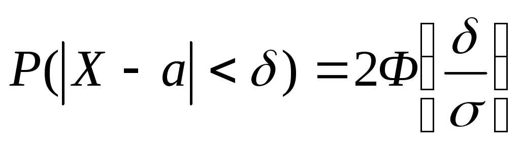. (4)

Substituting the available data into (4), we obtain:

Therefore, the probability that the length of the manufactured parts will be in the range from 39.4 to 40.6 cm is 0.8664.

Example. The diameter of parts manufactured by a plant is a random variable distributed according to a normal law. Standard Diameter Length a=2.5 cm, standard deviation σ=0.01. Within what limits can one practically guarantee the length of the diameter of this part if an event with a probability of 0.9973 is taken as reliable?

Solution. According to the conditions of the problem we have:

a=2.5; σ=0.01; .

Applying formula (4), we obtain the equality:

or
.

From Table 2 we find that the Laplace function has this value at x=3. Hence,
; whence σ=0.03.

In this way, it can be guaranteed that the diameter length will vary between 2.47 and 2.53 cm.

Laplace's integral theorem

Theorem. If the probability p of the occurrence of event A in each trial is constant and different from zero and one, then the probability that the number m of the occurrence of event A in n independent trials lies in the range from a to b (inclusive), with a sufficiently large number of trials n is approximately equal to

The integral formula of Laplace, as well as the local formula of Moivre-Laplace, the more accurate the more n and the closer to 0.5 the value p And q. Calculation using this formula gives an insignificant error if the condition is met npq≥ 20, although the fulfillment of the condition can be considered acceptable npq > 10.

Function Ф( x) tabulated (see Appendix 2). To use this table you need to know the properties of the function Ф( x):

1. Function Ф( x) – odd, i.e. F(– x) = – Ф( x).

2. Function Ф( x) – monotonically increasing, and as x → +∞ Ф( x) → 0.5 (practically we can assume that already at x≥ 5 F( x) ≈ 0,5).

Example 3.4. Using the conditions of Example 3.3, calculate the probability that from 300 to 360 (inclusive) students will successfully pass the exam the first time.

Solution. We apply Laplace's integral theorem ( npq≥ 20). We calculate:

= –2,5; = 5,0;

P 400 (300 ≤ m≤ 360) = Ф(5.0) – Ф(–2.5).

Taking into account the properties of the function Ф( x) and using the table of its values, we find: Ф(5,0) = 0.5; Ф(–2.5) = – Ф(2.5) = – 0.4938.

We get P 400 (300 ≤ m ≤ 360) = 0,5 – (– 0,4938) = 0,9938. ◄

Let us write down the consequences of Laplace's integral theorem.

Corollary 1. If the probability p of the occurrence of event A in each trial is constant and different from zero and one, then with a sufficiently large number n of independent trials, the probability that the number m of the occurrence of event A differs from the product np by no more than ε > 0

(3.8)

Example 3.5. Under the conditions of Example 3.3, find the probability that from 280 to 360 students will successfully pass the probability theory exam the first time.

Solution. Calculate probability R 400 (280 ≤ m≤ 360) can be similar to the previous example using the basic integral formula of Laplace. But it’s easier to do this if you notice that the boundaries of the interval 280 and 360 are symmetrical with respect to the value n.p.=320. Then, based on Corollary 1, we obtain

= = ≈

≈ = 2Ф(5.0) ≈ 2·0.5 ≈ 1,

those. It is almost certain that between 280 and 360 students will successfully pass the exam the first time. ◄

Corollary 2. If the probability p of the occurrence of event A in each trial is constant and different from zero and one, then with a sufficiently large number n of independent trials, the probability that the frequency m/n of event A lies in the range from α to β (inclusive) is equal to

(3.9)

Where

, .

(3.10)

Example 3.6. According to statistics, on average 87% of newborns live to be 50 years old. Find the probability that out of 1000 newborns the proportion (frequency) of those surviving to 50 years will be in the range from 0.9 to 0.95.

Solution. The probability that a newborn will live to be 50 years old is r= 0.87. Because n= 1000 is large (i.e. the condition npq= 1000·0.87·0.13 = 113.1 ≥ 20 satisfied), then we use Corollary 2 of Laplace’s integral theorem. We find:

2,82, = 7,52.

= 0,5 – 0,4976 = 0,0024. ◄

Corollary 3. If the probability p of the occurrence of event A in each trial is constant and different from zero and one, then with a sufficiently large number n of independent trials, the probability that the frequency m/n of event A differs from its probability p by no more thanΔ > 0 (in absolute value) equals

(3.11)

Example 3.7. According to the conditions of the previous problem, find the probability that out of 1000 newborns, the proportion (frequency) of those surviving to 50 years will differ from the probability of this event by no more than 0.04 (in absolute value).

Solution. Using Corollary 3 of Laplace’s integral theorem, we find:

= 2F(3.76) = 2·0.4999 = 0.9998.

Since inequality is equivalent to inequality, this result means that it is almost certain that from 83 to 91% of newborns out of 1000 will live to be 50 years old. ◄

Previously, we established that for independent trials the probability of the number m occurrences of the event A V n test is found using Bernoulli's formula. If n is large, then use Laplace's asymptotic formula. However, this formula is unsuitable if the probability of the event is small ( r≤ 0.1). In this case ( n great, r little) apply Poisson's theorem

Poisson's formula

Theorem. If the probability p of the occurrence of event A in each trial tends to zero (p → 0) with an unlimited increase in the number n of trials (n→ ∞), and the product np tends to a constant number λ (np → λ), then the probability P n (m) that event A will appear m times in n independent trials satisfies the limit equality

Local theorem of Moivre-Laplace(1730 Moivre and Laplace)

If the probability $p$ of occurrences of event $A$ is constant and $p\ne 0$ and $p\ne 1$, then the probability $P_n (k)$ is that event $A$ will appear $k$ times in $n $ tests, is approximately equal (the larger $n$, the more accurate) the value of the function $y=\frac ( 1 ) ( \sqrt ( n\cdot p\cdot q ) ) \cdot \frac ( 1 ) ( \sqrt ( 2 \pi ) ) \cdot e^ ( - ( x^2 ) / 2 ) =\frac ( 1 ) ( \sqrt ( n\cdot p\cdot q ) ) \cdot \varphi (x)$

for $x=\frac ( k-n\cdot p ) ( \sqrt ( n\cdot p\cdot q ) ) $. There are tables containing the values of the function $\varphi (x)=\frac ( 1 ) ( \sqrt ( 2\cdot \pi ) ) \cdot e^ ( - ( x^2 ) / 2 ) $

so \begin(equation) \label ( eq2 ) P_n (k)\approx \frac ( 1 ) ( \sqrt ( n\cdot p\cdot q ) ) \cdot \varphi (x)\,\,where\,x =\frac ( k-n\cdot p ) ( \sqrt ( n\cdot p\cdot q ) ) \qquad (2) \end(equation)

function $\varphi (x)=\varphi (( -x ))$ is even.

Example. Find the probability that event $A$ will occur exactly 80 times in 400 trials if the probability of this event occurring in each trial is $p=0.2$.

Solution. If $p=0.2$ then $q=1-p=1-0.2=0.8$.

$P_ ( 400 ) (( 80 ))\approx \frac ( 1 ) ( \sqrt ( n\cdot p\cdot q ) ) \varphi (x)\,\,where\,x=\frac ( k-n\cdot p ) ( \sqrt ( n\cdot p\cdot q ) ) $

$ \begin(array) ( l ) x=\frac ( k-n\cdot p ) ( \sqrt ( n\cdot p\cdot q ) ) =\frac ( 80-400\cdot 0.2 ) ( \sqrt ( 400 \cdot 0.2\cdot 0.8 ) ) =\frac ( 80-80 ) ( \sqrt ( 400\cdot 0.16 ) ) =0 \\ \varphi (0)=0.3989\,\,P_ ( 400 ) (( 80 ))\approx \frac ( 0.3989 ) ( 20\cdot 0.4 ) =\frac ( 0.3989 ) ( 8 ) =0.0498 \\ \end(array) $

Moivre-Laplace integral theorem

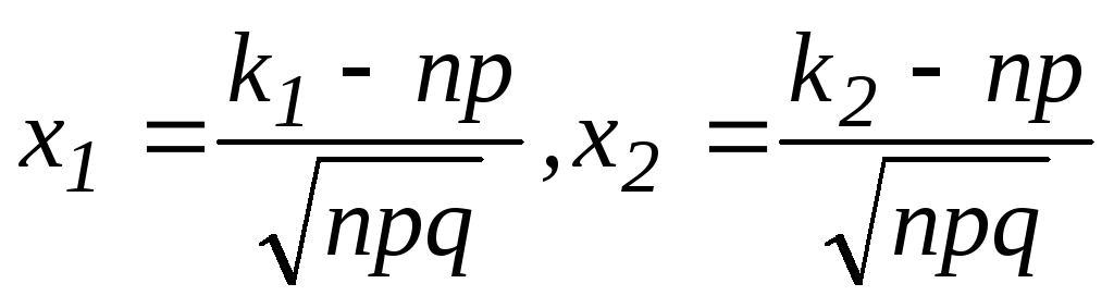
The probability P of the occurrence of event $A$ in each trial is constant and $p\ne 0$ and $p\ne 1$, then the probability $P_n (( k_1 ,k_2 ))$ that the event $A$ will occur from $k_ ( 1 ) $ up to $k_ ( 2 ) $ times in $n$ trials, equals $ P_n (( k_1 ,k_2 ))\approx \frac ( 1 ) ( \sqrt ( 2\cdot \pi ) ) \int\limits_ ( x_1 ) ^ ( x_2 ) ( e^ ( - ( z^2 ) / 2 ) dz ) =\Phi (( x_2 ))-\Phi (( x_1 ))$

where $x_1 =\frac ( k_1 -n\cdot p ) ( \sqrt ( n\cdot p\cdot q ) ) , x_2 =\frac ( k_2 -n\cdot p ) ( \sqrt ( n\cdot p\cdot q ) ) $ ,where

$\Phi (x)=\frac ( 1 ) ( \sqrt ( 2\cdot \pi ) ) \int ( e^ ( - ( z^2 ) / 2 ) dz ) $ -found from tables

$\Phi (( -x ))=-\Phi (x)$-odd

Odd function. The values in the table are given for $x=5$, for $x>5,\Phi (x)=0.5$

Example. It is known that 10% of products are rejected during inspection. 625 products were selected for control. What is the probability that among those selected there are at least 550 and at most 575 standard products?

Solution. If there are 10% defects, then there are 90% standard products. Then, by condition, $n=625, p=0.9, q=0.1, k_1 =550, k_2 =575$. $n\cdot p=625\cdot 0.9=562.5$. We get $ \begin(array) ( l ) P_ ( 625 ) (550.575)\approx \Phi (( \frac ( 575-562.5 ) ( \sqrt ( 625\cdot 0.9\cdot 0.1 ) ) ) )- \Phi (( \frac ( 550-562.5 ) ( \sqrt ( 626\cdot 0.9\cdot 0.1 ) )) \approx \Phi (1.67)- \Phi (-1, 67)=2 \Phi (1.67)=0.9052 \\ \end(array) $

If the probability of an event occurring in each test is constant and satisfies the double inequality
, and the number of independent trials is high enough, then the probability
can be calculated using the following approximate formula

(14) ,

where the limits of the integral are determined by the equalities

Formula (14) is more accurate the greater the number of tests in a given experiment.

Based on equality (13), formula (14) can be rewritten as

(15)
.

(16)
(N.F.L)

Let us note the simplest properties of the function
:

The last property is related to the properties of the Gaussian function
.

Function
odd. Indeed, after changing variables

=

;

To check the second property, it is enough to make a drawing. Analytically it is related to the so-called improper Poisson integral.

It directly follows from this that for all numbers
it can be assumed that
therefore, all values of this function are located in the interval [-0.5; 0.5], with the smallest being
then the function slowly grows and goes to zero, i.e.
and then increases to
Consequently, on the entire number line it is a strictly increasing function, i.e. If
That

It should be noted that the outputs of property 2 for the function
is justified on the basis of an improper Poisson integral.

Comment. When solving problems that require the application of the Moivre-Laplace integral theorem, special tables are used. The table shows the values for positive arguments and for
; for values
you should use the same table taking into account the equality

Next, in order to use the function table
, we transform equality (15) as follows:

And based on property 2 (odd parity
), taking into account the parity of the integrand we obtain

=
.

Thus, the probability that an event will appear in independent tests no less once and no more times, calculated by the formula:

(17)

;

Example 12. The probability of hitting the target with one shot is 0.75. Find the probability that with 300 shots the target will be hit at least 150 and not more than 250 times.

Solution: Here
,
,
,
,
. We calculate

,
,

,
.

Substituting into the Laplace integral formula, we get

In practice, along with equality (16), another formula is often used called “ probability integral"or the Laplace function (see in more detail in Chapter 2., paragraph 9., Vol. 9.).

(I.V. or F.L.)

For this function the equalities are valid:

Therefore, it is related to the tabulated function
and therefore there is also a table of approximate values (see appendix at the end of the book).

Example 13. The probability that the part did not pass the quality control inspection is 0.2. Find the probability that among 400 randomly selected untested parts there will be from 70 to 100 parts.

Solution. According to the conditions of the problem
,
,
.
,
. Let's use the Moivre-Laplace integral theorem:

Let's calculate the lower and upper limits of integration:

Therefore, taking into account the table values of the function
;

we get the required probability

Now we have the opportunity, as an application of the considered limit theorems, to prove the well-known theorem « law of large numbers in Bernoulli form »

Law of Large Numbers (LBA in Bernoulli form)

The first historically simplest law of large numbers is the theorem

J. Bernoulli. Bernoulli's theorem expresses the simplest form of the law of large numbers. It justifies the theoretical possibility of approximate calculation of the probability of an event using its relative frequency, i.e. substantiates the property of relative frequency stability.

Let it be carried out independent trials, in each of which the probability of the event occurring equal to
and the relative frequency in each test series is

Let's consider the problem:under test conditions according to the Bernoulli scheme and with a sufficiently large number of independent testsfind the probability of relative frequency deviation
from constant probability occurrence of an event in absolute value does not exceed a given number
In other words, find the probability:

with a sufficiently large number of independent tests.

Theorem (ZBCH J. Bernoulli 1713)Under the above conditions for any , no matter how little
, there is a limiting equality

(19)
.

Proof. Let us carry out the proof of this important statement based on the Moivre–Laplace integral theorem. By definition, the relative frequency is

A
probability of occurrence of an event in one test. First we establish the following equality for any
and big enough :

(20)

.

Indeed, in accordance with the condition
It is easy to see that there is a double inequality. Let's denote

(21)
.

Then, we will have the inequalities

Therefore, for the desired probability . Now, for cases
let's use the equality

;

and taking into account the odd number
we get

== 2
.

Equality (20) is obtained.

From formula (20) it immediately follows that when
(taking into account
where), we obtain limit equality (20).

Example 14.
. Find the probability that among 400 parts randomly selected, the relative frequency of occurrence of non-standard parts will deviate from
in absolute value by no more than 0.03.

Solution. According to the conditions of the problem, you need to find

According to formula (3) we have

=2
.

Taking into account the table value of the function
we get

The meaning of the result obtained is as follows: if you take a sufficiently large number of samples

details, then in each sample there is approximately a deviation of the relative “frequency” by

95.44% and value
of these samples from the probability
, modulo not exceeding 0.03.

Let's look at another example where you need to find a number
.

Example 15. The probability that a part is non-standard is
. How many parts must be selected so that with a probability of 0.9999 it can be stated that the relative frequency of non-standard parts (among those selected) deviates from modulo no more than 0.03. Find this quantity

Solution. Here, by condition
.

Need to determine
. According to formula (13) we have

Since,

From the table we find that this value corresponds to the argument
. From here,
. The meaning of this result is that the relative frequency will be concluded

between numbers. Thus, the number of non-standard parts in 99.99% of samples will be between the numbers 101.72 (7% of 1444) and 187.72 (13% of 1444).

If we take only one sample of 1444 parts, then with great confidence we can expect that the number of non-standard parts will be no less than 101 and no more than 188, while at the same time it is unlikely that there will be less than 101 or more than 188.

It should be noted that Bernoulli's theorem also states: with an unlimited increase in the number of trials, the frequency of a random event converges in probability to the true probability of the same event, i.e. the lower estimate is valid

(22)
;
,

provided that the probability of the event remains unchanged and equal from test to test
at the same time
.

Inequality (22) is a direct consequence of the well-known Chebyshev inequality (see further the topic “Limit theorems of probability theory” “Chebyshev’s theorem”). We will return to this BCA later. It is convenient for obtaining probability estimates from below and a two-sided estimate for the required number of occurrences of an event, so that the probability from the modulus of the difference between the relative frequency and the true probability satisfies the given constraint of the event under consideration.

Example 16. A coin is tossed 1000 times. Estimate from below the probability of deviation of the frequency of occurrence of a “coat of arms” from the probability of its occurrence by less than 0.1.

Solution. According to the condition here

Based on inequality (4), we obtain

Therefore the inequality
is equivalent to double inequality

Therefore, we can conclude that the probability of the number of hits of the “coat of arms” in the interval (400; 600) is greater than

Example 17. There are 1000 white and 2000 black balls in an urn. 300 balls were retrieved (with return). Estimate from below the probability that the number of balls drawn m(they must be white) satisfies the double inequality 80< m <120.

Solution. Double inequality for quantity m let's rewrite it in the form: