Fitting curves and surfaces to data using regression, interpolation and smoothing
Curve Fitting Toolbox™ provides the application and functionality for fitting curves and surfaces to data. The toolbox allows you to perform exploratory data analysis, pre-process and post-process data, compare candidate models, and remove outliers. You can perform regression analysis using the library of linear and nonlinear models provided, or you can define your own equations. The library provides optimized solver parameters and starting conditions to improve the quality of your fits. The toolbox also supports non-parametric modeling techniques such as splines, interpolation and smoothing.
Once the fit is created, a variety of post-processing techniques can be applied for plotting, interpolation, and extrapolation; assessment of confidence intervals; and calculating integrals and derivatives.
Getting started
Learn the basics of Curve Fitting Toolbox
Linear and nonlinear regression
Fit curves or surfaces with linear and nonlinear library models and custom models
Interpolation
Fit interpolation curves or surfaces, estimate values between known data points
Smoothing
Suitable smoothing uses slot and localized regression, smoothed data with moving average and other filters
Suitable post-processing
Graphical output, outliers, residuals, confidence intervals, validation data, integrals and derivatives, generates MATLAB ® code
Splines
Create splines with or without data; ppform, B-form, tensor product, rational, and stform thin plate splines
Lagrange polynomial
Lagrange interpolation polynomial- a polynomial of minimal degree that takes given values at a given set of points. For n+ 1 pairs of numbers, where everything x i are different, there is a unique polynomial L(x) degrees no more n, for which L(x i) = y i .
In the simplest case ( n= 1) is a linear polynomial whose graph is a straight line passing through two given points.
Definition
This example shows the Lagrange interpolation polynomial for the four points (-9,5) , (-4,2) , (-1,-2) and (7,9) , as well as the polynomials y j l j (x), each of which passes through one of the selected points, and takes a zero value in the rest x i
Let for the function f(x) values are known y j = f(x j) at some points. Then we can interpolate this function as

In particular,

Values of integrals from l j do not depend on f(x) and they can be calculated in advance, knowing the sequence x i .
For the case of uniform distribution of interpolation nodes over a segment
In this case we can express x i through the distance between interpolation nodes h and the starting point x 0 :
and therefore
.Substituting these expressions into the formula of the basic polynomial and taking h out of the multiplication signs in the numerator and denominator, we obtain

Now you can introduce a variable change
and get a polynomial from y, which is constructed using only integer arithmetic. The disadvantage of this approach is the factorial complexity of the numerator and denominator, which requires the use of algorithms with multi-byte representation of numbers.
External links
Wikimedia Foundation. 2010.
See what a “Lagrange polynomial” is in other dictionaries:
Form of notation of a polynomial of degree n (Lagrange interpolation polynomial), interpolating a given function f(x). at nodes x 0, x1,..., x n: In the case when the values of x i are equidistant, i.e. using the notation (x x0)/h=t formula (1)… … Mathematical Encyclopedia
In mathematics, polynomials or polynomials in one variable are functions of the form where ci are fixed coefficients and x is a variable. Polynomials constitute one of the most important classes of elementary functions. Study of polynomial equations and their solutions... ... Wikipedia
In computational mathematics, Bernstein polynomials are algebraic polynomials that are a linear combination of basic Bernstein polynomials. A stable algorithm for calculating polynomials in Bernstein form is the algorithm... ... Wikipedia
A polynomial of minimum degree that takes given values at a given set of points. For pairs of numbers where all are different, there is a unique polynomial of degree at most for which. In the simplest case (... Wikipedia
Lagrange interpolation polynomial A polynomial of minimum degree that takes given values at a given set of points. For n + 1 pairs of numbers, where all xi are different, there is a unique polynomial L(x) of degree at most n, for which L(xi) = yi.... ... Wikipedia
Lagrange interpolation polynomial A polynomial of minimum degree that takes given values at a given set of points. For n + 1 pairs of numbers, where all xi are different, there is a unique polynomial L(x) of degree at most n, for which L(xi) = yi.... ... Wikipedia
About the function, see: Interpolant. Interpolation in computational mathematics is a method of finding intermediate values of a quantity from an existing discrete set of known values. Many of those who deal with scientific and engineering calculations often... Wikipedia
About the function, see: Interpolant. Interpolation, interpolation in computational mathematics is a method of finding intermediate values of a quantity from an existing discrete set of known values. Many of those who encounter scientific and... ... Wikipedia
We will construct an interpolation polynomial in the form
where are polynomials of degree not higher than p, having the following property:
Indeed, in this case the polynomial (4.9) at each node x j, j=0,1,…n, is equal to the corresponding function value y j, i.e. is interpolative.
Let's construct such polynomials. Since at x=x 0 ,x 1 ,…x i -1 ,x i +1 ,…x n , we can factorize as follows
where c is a constant. From the condition we obtain that
Interpolation polynomial (4.1), written in the form
is called the Lagrange interpolation polynomial.
Approximate value of a function at a point x*, calculated using the Lagrange polynomial, will have a residual error (4.8). If the function values y i at interpolation nodes x i are given approximately with the same absolute error, then instead of the exact value, the approximate value will be calculated, and
where is the computational absolute error of the Lagrange interpolation polynomial. Finally, we have the following estimate of the total error of the approximate value.
In particular, the Lagrange polynomials of the first and second degrees will have the form
and their total errors at point x *
There are other forms of writing the same interpolation polynomial (4.1), for example, Newton's interpolation formula with divided differences and its variants considered below. When accurately calculating the value Pn(x *), obtained from different interpolation formulas constructed using the same nodes, coincide. The presence of a computational error leads to differences in the values obtained from these formulas. Writing a polynomial in Lagrange form usually leads to a smaller computational error.
The use of formulas for estimating errors arising during interpolation depends on the formulation of the problem. For example, if the number of nodes is known, and the function is given with a sufficiently large number of correct signs, then we can set the task of calculating f(x *) with the highest possible accuracy. If, on the contrary, the number of correct signs is small and the number of nodes is large, then we can pose the problem of calculating f(x *) with the accuracy that the table value of the function allows, and to solve this problem, both rarefaction and compaction of the table may be required.
§4.3. Separated differences and their properties.
The concept of a divided difference is a generalized concept of a derivative. Let the values of the functions be given at points x 0 , x 1 ,…x n f(x 0), f(x 1),…,f(x n). Divided differences of the first order are defined by the equalities
separated second order differences by equalities,
and the divided differences k th order are determined by the following recurrent formula:
The divided differences are usually placed in a table like this:
| x i | f(x i) | Divided differences | |||
| I order | II order | III order | IV order | ||
| x 0 | y 0 | ||||
| f | |||||
| x 1 | y 1 | f | |||
| f | f | ||||
| x 2 | y 2 | f | f | ||
| f | f | ||||
| x 3 | y 3 | f | |||
| f | |||||
| x 4 | y 4 |
Consider the following properties of divided differences.
1. Divided differences of all orders are linear combinations of values f(x i), i.e. the following formula holds:
Let us prove the validity of this formula by induction on the order of differences. For first order differences
Formula (4.12) is correct. Let us now assume that it is valid for all differences of order .
Then, according to (4.11) and (4.12) for differences of order k=n+1 we have
Terms containing f(x 0) And f(x n +1), have the required form. Let us consider the terms containing f(x i), i=1, 2, …,n. There are two such terms - from the first and second sums:
those. formula (4.12) is valid for a difference of order k=n+1, the proof is complete.
2. The divided difference is a symmetric function of its arguments x 0 , x 1 ,…x n (i.e. it does not change with any rearrangement):
This property follows directly from equality (4.12).
3. Simple divided difference relationship f and derivative f(n)(x) gives the following theorem.
Let nodes x 0 , x 1 ,…x n belong to the segment and function f(x) has on this interval a continuous derivative of the order n. Then there is such a point xÎ, What
Let us first prove the validity of the relation
According to (4.12), the expression in square brackets is
f.
From comparison (4.14) with expression (4.7) for the remainder term R n (x)=f(x)-L n (x) we obtain (4.13), the theorem is proven.
A simple corollary follows from this theorem. For a polynomial n th degree
f(x) = a 0 x n +a 1 x n -1 +…a n
order derivative n, obviously there is
and relation (4.13) gives for the divided difference the value
So, every polynomial has degrees n separated order differences n are equal to a constant value - the coefficient of the highest degree of the polynomial. Separated differences of higher orders
(more n), are obviously equal to zero. However, this conclusion is valid only if there is no computational error in the separated differences.
§4.4. Newton's divided difference interpolation polynomial
Let us write the Lagrange interpolation polynomial in the following form:
Where L 0 (x) = f(x 0)=y 0, A Lk(x)– Lagrange interpolation polynomial of degree k, built by nodes x 0 , x 1 , …,x k. Then there is a polynomial of degree k, whose roots are points x 0 , x 1 , …,x k -1. Therefore, it can be factorized
where A k is a constant.
In accordance with (4.14) we obtain
Comparing (4.16) and (4.17) we find that (4.15) also takes the form
which is called Newton's divided difference interpolation polynomial.
This type of recording of the interpolation polynomial is more visual (the addition of one node corresponds to the appearance of one term) and allows us to better trace the analogy of the constructions being carried out with the basic constructions of mathematical analysis.
The residual error of the Newton interpolation polynomial is expressed by formula (4.8), but, taking into account (4.13), it can be written in another form
those. the residual error can be estimated by the modulus of the first discarded term in the polynomial Nn(x*).
Computational error Nn(x*) will be determined by the errors of the separated differences. Interpolation nodes closest to the interpolated value x*, will have a greater influence on the interpolation polynomial, those lying further away will have a lesser influence. It is therefore advisable, if possible, to x 0 And x 1 take the ones closest to x* interpolation nodes and first perform linear interpolation along these nodes. Then gradually attract the following nodes so that they are located as symmetrically as possible relative to x*, until the next term in absolute value is less than the absolute error of the divided difference included in it.
In computing practice, one often has to deal with functions specified by tables of their values for some finite set of values X : .
In the process of solving the problem, it is necessary to use the values
 for intermediate argument values. In this case, construct a function Ф(x), simple enough for calculations, which at given points x 0
, x 1
,...,x n ,
called interpolation nodes, takes values, and at the remaining points of the segment (x 0 ,x n) belonging to the domain of definition
for intermediate argument values. In this case, construct a function Ф(x), simple enough for calculations, which at given points x 0
, x 1
,...,x n ,
called interpolation nodes, takes values, and at the remaining points of the segment (x 0 ,x n) belonging to the domain of definition
 , approximately represents the function
 with varying degrees of accuracy.
When solving the problem in this case, instead of the function
 operate with the function Ф(x). The problem of constructing such a function Ф(x) is called the interpolation problem. Most often, the interpolating function Ф(x) is found in the form of an algebraic polynomial.
Interpolation polynomial
For every function
 , defined on [ a,b], and any set of nodes x 0
, x 1
,....,x n (x i
, defined on [ a,b], and any set of nodes x 0
, x 1
,....,x n (x i
 [a,b],
x i
[a,b],
x i  x j at i
 j) among algebraic polynomials of degree no higher than n, there is a unique interpolation polynomial Ф(x), which can be written in the form:
 ,
(3.1)
,
(3.1)
Where  - a polynomial of nth degree having the following property:
For an interpolation polynomial, the polynomial  has the form:
This polynomial (3.1) solves the interpolation problem and is called the Lagrange interpolation polynomial.
As an example, consider a function of the form  on the interval
  specified in a tabular manner.
It is necessary to determine the value of the function at point x-2.5. Let's use the Lagrange polynomial for this. Based on formulas (3.1 and 3.3), we write this polynomial in explicit form:
 (3.4).
Then, substituting the initial values from our table into formula (3.4), we obtain
The obtained result corresponds to the theory i.e. .
Lagrange interpolation formula
The Lagrange interpolation polynomial can be written in another form:
 (3.5)
(3.5)
Writing a polynomial in the form (3.5) is more convenient for programming.
When solving the interpolation problem, the quantity n is called the order of the interpolating polynomial. In this case, as can be seen from formulas (3.1) and (3.5), the number of interpolation nodes will always be equal to n+1 and meaning x,
for which the value is determined
 ,
must lie inside the definition area of the interpolation nodes
those.
,
must lie inside the definition area of the interpolation nodes
those.
 . (3.6)
In some practical cases, the total known number of interpolation nodes m may be greater than the order of the interpolating polynomial n.
In this case, before implementing the interpolation procedure according to formula (3.5), it is necessary to determine those interpolation nodes for which condition (3.6) is valid. It should be remembered that the smallest error is achieved when finding the value x in the center of the interpolation area. To ensure this, the following procedure is suggested:

The main purpose of interpolation is to calculate the values of a tabulated function for non-nodal (intermediate) argument values, which is why interpolation is often called “the art of reading tables between rows.”
We will look for an interpolation polynomial in the form
VANDERMOND ALEXANDER THEOPHILE (Vandermonde Alexandre Theophill; 1735-1796) - French mathematician whose main works relate to algebra. V. laid the foundations and gave a logical presentation of the theory of determinants (Vandermonde determinant), and also isolated it from the theory of linear equations. He introduced the rule for the expansion of determinants using second-order minors.
Here 1.(x)- polynomials of degree n, the so-called LAGRANGEAN INFLUENCE POLYNOMIALS, satisfying the condition

The last condition means that any polynomial l t (x) equals zero for every x-y except X. at i.e. x 0 y x v ...» x ( _ v x i + v ...» x n are the roots of this polynomial. Therefore, the Lagrangian polynomials Ifjx) look like
Since by condition 1.(x.) = 1, then
Thus, the Lagrangian influence polynomials will be written in the form

and the interpolation polynomial (2.5) will be written in the form
LAGRANGE JOSEPH LOUIS (Lagrange Joseph Louis; 1736-1813) - an outstanding French mathematician and mechanic, whose most important works relate to the calculus of variations, analytical and theoretical mechanics. L.'s statics was based on the principle of possible (virtual) movements. He introduced generalized coordinates and gave the equations of motion of a mechanical system the form named after him. L. obtained a number of important results in the field of analysis (the formula for the remainder of the Taylor series, the formula for finite increments, the theory of conditional extrema); in theory numbers(Lagrange's theorem); in algebra (the theory of continued fractions, reducing the quadratic form to the sum of squares); in the theory of differential equations (finding the quotient solutions the study of a first-order ordinary differential equation, linear with respect to the desired function and an independent variable, with variable coefficients depending on the derivative of the desired function); in the theory of interpolation (Lagrange interpolation formula).
The interpolation polynomial in the form (2.6) is called the LAGRANGE INTERPOLATION POLYNOMIAL. Let us list the main advantages of this form of writing the interpolation polynomial.
- The number of arithmetic operations required to construct a Lagrange polynomial is proportional to n 2 and is the smallest for all notation forms.
- Formula (2.6) explicitly contains the values of the functions at the interpolation nodes, which is convenient for some calculations, in particular, when constructing numerical integration formulas.
- Formula (2.6) is applicable for both equally spaced and unequally spaced nodes.
- The Lagrange interpolation polynomial is especially useful when the function values change but the interpolation nodes remain unchanged, which is the case in many experimental studies.
The disadvantages of this form of recording include the fact that with a change in the number of nodes, all calculations have to be carried out again. This makes it difficult to make a posteriori estimates of accuracy (estimates obtained during the calculation process).
Let us introduce the function ω l f , = (x - x 0)(x - Xj)...(x - x p)=fl(*“*;)
Note that w n + : (x) is degree polynomial n + 1. Then formula (2.6) can be written in the form
Here are the formulas for linear and quadratic interpolation according to Lagrange:

The Lagrange polynomial is a polynomial of the 1st degree in formula (2.8) and a polynomial of the 2nd degree in formula (2.9).
These formulas are most often used in practice. Let given (n + 1) interpolation unit. At these nodes one can construct one interpolation polynomial n th degree, (p - 1) a polynomial of the first degree and a large set of polynomials of degree less p, based on some of these nodes. Theoretically, higher degree polynomials provide maximum accuracy. However, in practice, polynomials of low degrees are most often used to avoid errors when calculating coefficients for large degrees of the polynomial.