During calculations, sometimes you need to add percentages to a specific number. For example, to find out the current profit indicators, which have increased by a certain percentage compared to the previous month, you need to add this percentage to the profit of the previous month. There are many other examples where you need to perform a similar action. Let's figure out how to add a percentage to a number in Microsoft Excel.
So, if you just need to find out what a number will be equal to after adding a certain percentage to it, then you should enter an expression using the following template in any cell of the sheet, or in the formula bar: “=(number)+(number)*(percentage_value )%".
Let's say we need to calculate what number we get if we add twenty percent to 140. Write the following formula in any cell, or in the formula bar: “=140+140*20%”.


Applying a formula to actions in a table
Now, let's figure out how to add a certain percentage to the data that is already in the table.
First of all, select the cell where the result will be displayed. We put a “=” sign in it. Next, click on the cell containing the data to which the percentage should be added. We put the “+” sign. Again, click on the cell containing the number and put the “*” sign. Next, we type on the keyboard the percentage by which the number should be increased. Don’t forget to put the “%” sign after entering this value.

Click on the ENTER button on the keyboard, after which the calculation result will be shown.

If you want to extend this formula to all the values of a column in the table, then simply stand on the lower right edge of the cell where the result is displayed. The cursor should turn into a cross. Click on the left mouse button, and with the button held down, “stretch” the formula down to the very end of the table.

As you can see, the result of multiplying numbers by a certain percentage is also displayed for other cells in the column.

We found that adding a percentage to a number in Microsoft Excel is not that difficult. However, many users do not know how to do this and make mistakes. For example, the most common mistake is to write a formula using the algorithm “=(number)+(percent_value)%” instead of “=(number)+(number)*(percentage_value)%”. This guide should help you avoid such mistakes.
In life, sooner or later everyone will be faced with a situation where it will be necessary to work with percentages. But, unfortunately, most people are not prepared for such situations. And this action causes difficulties. This article will tell you how to subtract percentages from a number. Moreover, various ways to solve the problem will be discussed: from the simplest (using programs) to one of the most complex (using a pen and paper).
We subtract manually
Now we will learn how to subtract with a pen and paper. The actions that will be presented below are studied by absolutely every person in school. But for some reason, not everyone remembered all the manipulations. So, we have already figured out what you will need. Now we'll tell you what needs to be done. To make it more clear, we will consider an example, taking specific numbers as a basis. Let's say you want to subtract 10 percent from the number 1000. Of course, it is quite possible to do these actions in your head, since the task is very simple. The main thing is to understand the very essence of the decision.
First of all, you need to write down the proportion. Let's say you have two columns with two rows. You need to remember one thing: numbers are entered in the left column, and percentages are entered in the right column. Two values will be written in the left column - 1000 and X. X is included because it symbolizes the number that will need to be found. In the right column will be entered - 100% and 10%.
Now it turns out that 100% is the number 1000, and 10% is X. To find x, you need to multiply 1000 by 10. Divide the resulting value by 100. Remember: the required percentage must always be multiplied by the taken number, after which the product should be divided by 100%. The formula looks like this: (1000*10)/100. The picture will clearly show all the formulas for working with percentages.
We got the number 100. This is what lies under that X. Now all that remains to be done is subtract 100 from 1000. It turns out 900. That's all. Now you know how to subtract percentages from a number using a pen and notebook. Practice on your own. And over time, you will be able to perform these actions in your mind. Well, we move on, talking about other methods.
Subtract using the Windows calculator
It’s clear: if you have a computer at hand, then few people will want to use a pen and notebook for calculations. It's easier to use technology. That’s why we’ll now look at how to subtract percentages from a number using a Windows calculator. However, it is worth making a small note: many calculators are capable of performing these actions. But the example will be shown using a Windows calculator for greater understanding.

Everything is simple here. And it is very strange that few people know how to subtract percentages from a number in a calculator. Initially, open the program itself. To do this, go to the Start menu. Next, select "All Programs", then go to the "Accessories" folder and select "Calculator".
Now everything is ready to start solving. We will operate with the same numbers. We have 1000. And we need to subtract 10% from it. All you need to do is enter the first number (1000) into the calculator, then press minus (-), and then click on percentage (%). Once you have done this, you will immediately see the expression 1000-100. That is, the calculator automatically calculated how much 10% of 1000 is.
Now press Enter or equals (=). Answer: 900. As you can see, both the first and second methods led to the same result. Therefore, it’s up to you to decide which method to use. Well, in the meantime we move on to the third and final option.
Subtract in Excel
Many people use Excel. And there are situations when it is vital to quickly make calculations in this program. That is why now we will figure out how to subtract a percentage from a number in Excel. This is very easy to do in the program using formulas. For example, you have a column with values. And you need to subtract 25% from them. To do this, select the column next to it and enter equal (=) in the formula field. After that, click LMB on the cell with the number, then put “-” (and again click on the cell with the number, after that enter - “*25%). You should get something like in the picture.

As you can see, this is the same formula as given the first time. After pressing Enter you will receive the answer. To quickly subtract 25% from all numbers in a column, just hover over the answer, placing it in the lower right corner, and drag down the required number of cells. Now you know how to subtract a percentage from a number in Excel.
Conclusion
Finally, I would like to say only one thing: as you can see from all of the above, in all cases only one formula is used - (x*y)/100. And it was with her help that we were able to solve the problem in all three ways.
Hi all! Do you know how to calculate percentages in Excel? In fact, percentages accompany us very often in life. After today's lesson, you will be able to calculate the profitability of an idea that suddenly arises, find out how much you actually get by participating in store promotions. Master some points and be on top of your game.
I'll show you how to use the basic calculation formula, calculate percentage growth, and other tricks.
This definition as a percentage is familiar to everyone from school. It comes from Latin and literally means “out of a hundred.” There is a formula that calculates percentages: 
Consider an example: there are 20 apples, 5 of which you gave to your friends. Determine in percentage what part did you give? Thanks to simple calculations we get the result: 
This is how percentages are calculated both at school and in everyday life. Thanks to Excel, such calculations become even easier, because everything happens automatically. There is no single formula for calculations. The choice of calculation method will also depend on the desired result.
How to calculate percentages in Excel: basic calculation formula
There is a basic formula that looks like:  Unlike school calculations, this formula does not need to multiply by 100. Excel takes care of this step, provided that the cells are assigned a certain percentage format.
Let's look at a specific example of the situation. There are products that are being ordered, and there are products that have been delivered. Order in column B, named Ordered. Delivered products are located in column C named Delivered. It is necessary to determine the percentage of fruit delivered:
- In cell D2, write the formula =C2/B2. Decide how many rows you need and, using autocomplete, copy it.
- In the “Home” tab, find the “Number” command, select “Percent Style”.
- Look at the decimal places. Adjust their quantity if necessary.
- All! Let's look at the result.
The last column D now contains values that show the percentage of orders delivered. 
How to calculate percentages of the total amount in Excel
Now we will look at some more examples of how how to calculate percentages in excel from the total amount, which will allow you to better understand and assimilate the material.
1.The calculated amount is located at the bottom of the table
At the end of the table you can often see the “Total” cell, where the total amount is located. We have to make the calculation of each part towards the total value. The formula will look like the previously discussed example, but the denominator of the fraction will contain an absolute reference. We will have the $ sign in front of the row and column names.
Column B is filled with values, and cell B10 contains their total. The formula will look like:  Using a relative reference in cell B2 will allow it to be copied and pasted into cells in the Ordered column.
2.Parts of the amount are located on different lines
Suppose we need to collect data that is located in different rows and find out what part is taken by orders for a certain product. Adding specific values is possible using the SUMIF function. The result we get will be necessary for us to calculate the percentage of the amount.
Column A is our range, and the summing range is in column B. We enter the product name in cell E1. This is our main criterion. Cell B10 contains the total for products. The formula takes on the following form: 

In the formula itself you can place the name of the product: 
If you need to calculate, for example, how much cherries and apples occupy as a percentage, then the amount for each fruit will be divided by the total. The formula looks like this:
Calculation of percentage changes
Calculating data that changes can be expressed as a percentage and is the most common task in Excel. The formula to calculate the percentage change is as follows: 
In the process of work, you need to accurately determine which of the meanings occupies which letter. If you have more of any product today, it will be an increase, and if less, then it will be a decrease. The following scheme works:
Now we need to figure out how we can apply it in real calculations.
1.Count changes in two columns
Let's say we have 2 columns B and C. In the first we display the prices of the month of the past, and in the second - of this month. To calculate the resulting changes, we enter a formula in column D. 
The calculation results using this formula will show us whether there is an increase or decrease in price. Fill in all the lines you need with the formula using autocomplete. For formula cells, be sure to activate the percentage format. If you did everything correctly, you get a table like this, where the increase is highlighted in black and the decrease in red. 
If you are interested in changes over a certain period and the data is in one column, then we use this formula: 
We write down the formula, fill in all the lines that we need and get the following table: 
If you want to count changes for individual cells, and compare them all with one, use the already familiar absolute reference, using the $ sign. We take January as the main month and calculate the changes for all months as a percentage: 
Copying a formula across other cells will not modify it, but a relative link will change the numbering.

Calculation of value and total amount by known percentage
I have clearly demonstrated to you that there is nothing complicated in calculating percentages through Excel, as well as in calculating the amount and values when the percentage is already known.
1.Calculate the value using a known percentage
For example, you buy a new phone that costs $950. You are aware of the VAT surcharge of 11%. It is necessary to determine the additional payment in monetary terms. This formula will help us with this: 
In our case, applying the formula =A2*B2 gives the following result: 
You can take either decimal values or using percentages.
2.Calculation of the total amount
Consider the following example, where the known original amount is $400, and the seller tells you that the price is now 30% less than last year. How to find out the original cost?
The price decreased by 30%, which means we need to subtract this figure from 100% to determine the required share: 
The formula that will determine the initial cost: 
Given our problem, we get: 

Converting a value to a percentage
This method of calculation is useful for those who especially carefully monitor their expenses and want to make some changes to them.
To increase the value by a percentage we will use the formula: 
We need to reduce the percentage. Let's use the formula: 
Using the formula =A1*(1-20%) reduces the value that is contained in a cell.
Our example shows a table with columns A2 and B2, where the first is the current expenses, and the second is the percentage by which you want to change expenses in one direction or another. Cell C2 should be filled with the formula: 

Increase by a percentage the values in a column
If you want to make changes to an entire data column without creating new columns and using an existing one, you need to do 5 steps:

Now we see values that have increased by 20%. 
Using this method, you can perform various operations on a certain percentage, entering it into a free cell.
Today was an extensive lesson. I hope you've made it clear How to calculate percentages in Excel. And, despite the fact that such calculations are not very popular for many, you will do them with ease.
Using a percentage calculator you can make all kinds of calculations using percentages. Rounds results to the required number of decimal places.
What percentage is number X of number Y. What number is X percent of number Y. Adding or subtracting percentages from a number.
Interest calculator
clear formHow much is % of number
Calculation0% of number 0 = 0
Interest calculator
clear formWhat % is the number from the number
CalculationNumber 15 from number 3000 = 0.5%
Interest calculator
clear formAdd % to number
CalculationAdd 0% to the number 0 = 0
Interest calculator
clear formSubtract % of the number
Calculation to clear everythingThe calculator is designed specifically for calculating interest. Allows you to perform a variety of calculations when working with percentages. Functionally it consists of 4 different calculators. See examples of calculations on the interest calculator below.
In mathematics, a percentage is one hundredth of a number. For example, 5% of 100 is 5.
This calculator will allow you to accurately calculate the percentage of a given number. There are various calculation modes available. You will be able to make various calculations using percentages.
- The first calculator is needed when you want to calculate the percentage of the amount. Those. Do you know the meaning of percentage and amount?
- The second one is if you need to calculate what percentage X is of Y. X and Y are numbers, and you are looking for the percentage of the first in the second
- The third mode is adding a percentage of the specified number to the given number. For example, Vasya has 50 apples. Misha brought Vasya another 20% of the apples. How many apples does Vasya have?
- The fourth calculator is the opposite of the third. Vasya has 50 apples, and Misha took 30% of the apples. How many apples does Vasya have left?
Frequent tasks
Task 1. An individual entrepreneur receives 100 thousand rubles every month. He works in a simplified manner and pays taxes of 6% per month. How much taxes does an individual entrepreneur have to pay per month?Solution: We use the first calculator. Enter the bet 6 in the first field, 100000 in the second
We receive 6,000 rubles. - tax amount.
Problem 2. Misha has 30 apples. He gave 6 to Katya. What percentage of the total number of apples did Misha give to Katya?
Solution: We use the second calculator - enter 6 in the first field, 30 in the second. We get 20%.
Task 3. At Tinkoff Bank, for replenishing a deposit from another bank, the depositor receives 1% on top of the replenishment amount. Kolya replenished the deposit with a transfer from another bank in the amount of 30,000. What is the total amount for which Kolya’s deposit will be replenished?
Solution: We use the 3rd calculator. Enter 1 in the first field, 10000 in the second. Click on the calculation and we get the amount of 10,100 rubles.
In this lesson, you will learn various useful formulas for adding and subtracting dates in Excel. For example, you will learn how to subtract another from one date, how to add several days, months or years to a date, etc.
If you have already taken lessons on working with dates in Excel (ours or any other lessons), then you should know the formulas for calculating units of time, such as days, weeks, months, years.
When analyzing dates in any data, you often need to perform arithmetic operations on these dates. This article will explain some formulas for adding and subtracting dates that you may find useful.
How to subtract dates in Excel
Let's assume that in your cells A2 And B2 contains dates, and you need to subtract one date from another to find out how many days there are between them. As is often the case in Excel, this result can be obtained in several ways.
Example 1. Directly subtract one date from another
I think you know that Excel stores dates as integers starting at 1, which corresponds to January 1, 1900. So you can simply arithmetically subtract one number from another:
Example 2: Subtracting dates using the DATEDAT function
If the previous formula seems too simple to you, the same result can be obtained in a more sophisticated way using the function RAZNDAT(DATEDIF).
RAZNDAT(A2;B2,"d")
=DATEDIF(A2,B2,"d")
The following figure shows that both formulas return the same result, except for row 4, where the function RAZNDAT(DATEDIF) returns an error #NUMBER!(#NUM!). Let's see why this happens.
When you subtract a later date (May 6, 2015) from an earlier date (May 1, 2015), the subtraction operation returns a negative number. However, the function syntax RAZNDAT(DATEDIF) does not allow start date was more end date and, of course, returns an error.
Example 3. Subtract the date from the current date
To subtract a specific date from the current date, you can use any of the previously described formulas. Just use the function instead of today's date TODAY(TODAY):
TODAY()-A2
=TODAY()-A2
RAZNDAT(A2;TODAY();"d")
=DATEDIF(A2,TODAY(),"d")
As in the previous example, the formulas work fine when the current date is greater than the subtracted date. Otherwise the function RAZNDAT(DATEDIF) returns an error.

Example 4: Subtracting Dates Using the DATE Function
If you prefer to enter dates directly into the formula, specify them using the function DATE(DATE) and then subtract one date from the other.
Function DATE has the following syntax: DATE( year; month; day) .
For example, the following formula subtracts May 15, 2015 from May 20, 2015 and returns the difference - 5 days.
DATE(2015,5,20)-DATE(2015,5,15)
=DATE(2015,5,20)-DATE(2015,5,15)

If necessary count the number of months or years between two dates, then the function RAZNDAT(DATEDIF) is the only possible solution. In the continuation of the article you will find several examples of formulas that reveal this function in detail.
Now that you know how to subtract one date from another, let's see how you can add or subtract a certain number of days, months or years from a date. There are several Excel functions for this. Which one to choose depends on what units of time need to be added or subtracted.
How to add (subtract) days to a date in Excel
If you have a date in a cell or a list of dates in a column, you can add (or subtract) a certain number of days to them using the appropriate arithmetic operation.
Example 1: Adding days to a date in Excel
The general formula for adding a certain number of days to a date is:
= Date + N days
The date can be set in several ways:
- Cell reference:
- Calling a function DATE(DATE):
DATE(2015;5;6)+10
=DATE(2015,5,6)+10 - Calling another function. For example, to add several days to the current date, use the function TODAY(TODAY):
TODAY()+10
=TODAY()+10
The following figure shows the operation of these formulas. At the time of writing, the current date was May 6, 2015.

Note: The result of these formulas is an integer representing a date. To show it as a date, you need to select the cell (or cells) and click Ctrl+1. A dialog box will open Cell Format(Format Cells). On the tab Number(Number) in the list of number formats, select Date(Date) and then specify the format you need. You will find a more detailed description in the article.
Example 2: Subtracting days from a date in Excel
To subtract a certain number of days from a date, you again need to use the normal arithmetic operation. The only difference from the previous example is minus instead of plus
= Date - N days
Here are some examples of formulas:
A2-10
=DATE(2015,5,6)-10
=TODAY()-10

How to add (subtract) several weeks to a date
When you need to add (subtract) several weeks to a certain date, you can use the same formulas as before. You just need to multiply the number of weeks by 7:
- Add N weeks to date in Excel:
A2+ N weeks * 7
For example, to add 3 weeks to a date in a cell A2, use the following formula:
- Subtract N weeks from date in Excel:
A2 - N weeks * 7
To subtract 2 weeks from today's date, use this formula:
TODAY()-2*7
=TODAY()-2*7
How to add (subtract) several months to a date in Excel
To add (or subtract) a certain number of months to a date, you need to use the function DATE(DATE) or DATAMES(EDATE) as shown below.
Example 1: Adding several months to a date using the DATE function
If the list of dates is, for example, in the column A, indicate the number of months that you want to add (positive number) or subtract (negative number) in some cell, say, in C2.
Type in cell B2 formula below, click on the highlighted corner of the cell and drag it down the column with the mouse B to the last filled cell in the column A. Formula from cell B2 will be copied to all cells of the column B.
DATE(YEAR(A2),MONTH(A2)+$C$2,DAY(A2))
=DATE(YEAR(A2),MONTH(A2)+$C$2,DAY(A2))

Let's see what this formula does. The logic of the formula is clear and obvious. Function DATE( year; month; day) receives the following arguments:
- Year from date in cell A2;
- Month from date in cell A2+ number of months indicated in the cell C2;
- Day from date in cell A2;
It's simple! If you enter in C2 negative number, the formula will subtract months rather than add.

Naturally, nothing prevents you from entering a minus directly in the formula to subtract months:
DATE(YEAR(A2),MONTH(A2)-$C$2,DAY(A2))
=DATE(YEAR(A2),MONTH(A2)-$C$2,DAY(A2))
And, of course, you can specify the number of months to add or subtract directly in the formula without cell reference. The finished formulas will look something like this:
- Add months to date:
DATE(YEAR(A2),MONTH(A2)+2,DAY(A2))
=DATE(YEAR(A2),MONTH(A2)+2,DAY(A2)) - Subtract months from date:
DATE(YEAR(A2),MONTH(A2)-2,DAY(A2))
=DATE(YEAR(A2),MONTH(A2)-2,DAY(A2))
Example 2: Adding or subtracting months from a date using the DATAMES function
Excel has a special function that returns a date that is a certain number of months ago or forward from a given date - this is the function DATAMES(EDATE). It is available in the latest versions of Excel 2007, 2010, 2013 and the new Excel 2016.
When using DATAMES(EDATE) You provide the following two arguments:
- Start date – the date from which the number of months is counted.
- Months – the number of months to be added (positive number) or subtracted (negative number).
These formulas will give the same result as formulas with the function DATE(DATE) in the previous example:

When using the function DATAMES(EDATE) the start date and number of months can be specified directly in the formula. Dates can be set using the function DATE(DATE) or as a result of executing other formulas. For example:
- This formula adds 10 months to May 7, 2015
DATAMES(DATE(2015,5,7),10)
=EDATE(DATE(2015,5,7),10) - This formula subtracts 10 months from today's date
DATAMES(TODAY();-10)
=EDATE(TODAY(),-10)
Note: Function DATAMES(EDATE) returns just an integer. To represent it as a date, you need to apply a date format to the cell. How to do this is indicated in the article How to change date format in Excel.
How to add (subtract) years to a date in Excel
Adding years to dates in Excel is the same as adding months. You need to use the function again DATE(DATE), but this time you need to specify the number of years you want to add:
DATE(YEAR( date) + N years; MONTH( date); DAY( date))
= DATE(YEAR( date) + N years,MONTH( date), DAY( date))
On an Excel worksheet, the formulas might look like this:
- Add 5 years to the date specified in the cell A2:
DATE(YEAR(A2)+5,MONTH(A2),DAY(A2))
=DATE(YEAR(A2)+5,MONTH(A2),DAY(A2)) - Subtract 5 years from the date specified in the cell A2:
DATE(YEAR(A2)-5,MONTH(A2),DAY(A2))
=DATE(YEAR(A2)-5,MONTH(A2),DAY(A2))
To get a universal formula, you can enter the number of years in a cell, and then refer to that cell in the formula. A positive number will add years to the date, and a negative number will subtract.

Adding (subtracting) days, months and years to a date
If you carefully read the two previous examples, then I think you figured out how to add (or subtract) years, months and days to a date in one formula. Yes, using the good old function DATE(DATA)!
- For additions X years, Y months and Z days:
DATE(YEAR( date) + X years; MONTH( date) + Y months; DAY( date) + Z days)
= DATE(YEAR( date) + X years,MONTH( date) + Y months, DAY( date) + Z days) - For subtraction X years, Y months and Z days:
DATE(YEAR( date) - X years; MONTH( date) - Y months; DAY( date) - Z days)
= DATE(YEAR( date) - X years,MONTH( date) - Y months, DAY( date) - Z days)
For example, the following formula adds 2 years and 3 months, and subtracts 15 days from the date in the cell A2:
DATE(YEAR(A2)+2;MONTH(A2)+3;DAY(A2)-15)
=DATE(YEAR(A2)+2,MONTH(A2)+3,DAY(A2)-15)
When applied to our date column, the formula takes the following form:
DATE(YEAR(A2)+$C$2,MONTH(A2)+$D$2,DAY(A2)+$E$2)
=DATE(YEAR(A2)+$C$2,MONTH(A2)+$D$2,DAY(A2)+$E$2)

How to Add and Subtract Time in Excel
In Microsoft Excel, you can add and subtract time using the function TIME(TIME). It allows you to handle units of time (hours, minutes and seconds) in the same way as years, months and days in the function DATE(DATE).
- Add time in Excel:
A2 + TIME( watch; minutes; seconds)
= A2 + TIME( watch, minutes, seconds) - Subtract time in Excel:
A2 - TIME( watch; minutes; seconds)
= A2 - TIME( watch, minutes, seconds)Where A2– this is a cell with the time that needs to be changed.
For example, to add 2 hours 30 minutes and 15 seconds to the time in a cell A2 you need to use the following formula:
A2+TIME(2;30;15)
=A2+TIME(2,30,15)
A2+TIME(2;30;-15)
=A2+TIME(2.30,-15)
You can also enter the desired values into the worksheet cells and refer to them in the formula:
A2+TIME($C$2,$D$2,$E$2)
=A2+TIME($C$2,$D$2,$E$2)