How to calculate GPA in Excel. How to find the average in Excel

If you need to determine the average revenue of your department for six months or calculate the average length of service of your company's employees, then you will need an arithmetic average in Excel. But if you have a lot of data, manually counting such actions will take a really long time. It is faster to do this using the special function AVERAGE(). Mastery of this formula is one of the fundamental elements of initial data analytics.

Usually in everyday life we ​​say that we need to calculate the average value, we mean that we need the arithmetic mean value in Excel (SA) - but there are quite a lot of average values ​​in mathematics.

We will try to discuss the most popular ones:

The simplest option. Arithmetic mean in Excel. AVERAGE function

How to use a formula involving AVERAGE? Everything is simple when you know;) Select the desired cell, put “=” in it and start writing AVERAGE, a formula will appear, as in the picture above. Select it with the mouse or the TAB key. You can call the desired command through the icon on the taskbar, the “Home” menu, find the autosum icon Σ, click and the line “Average” will appear on the right.
You have chosen the formula, now you need to indicate inside the opened brackets the range of cell values ​​whose average you want to calculate. If the participating cells are in a continuous array, then it is enough to select them at a time by dragging the borders with the left mouse button. When you need a separate selection, selecting specific cells, you need to select them by clicking on each one, and putting a semicolon between them ";"
Another way to activate any function is to access the standard Excel Function Wizard - the fx button (under the task ribbon) is responsible for it.

Pre-select a cell, then click on the fx button in the window that appears, find AVERAGE and confirm the selection using the “OK” or Enter button. You will be prompted for arguments involved in the calculation. Directly in this mode, the required areas of the table are selected, the selection is confirmed by pressing “Ok”, after which the calculation result will immediately appear in the marked field.

CA calculation based on a set of conditions

Firstly, for correct operation, you need to take into account that cells that are empty in value are not taken into account (that is, even 0 is not written there), they are completely excluded from the calculation.
Secondly, Excel directly works with 3 categories of arithmetic averages:

- simple average - the result of adding a set of numbers and then dividing the sum by the number of these numbers;
— median – a value that averagely characterizes the entire set of numbers;
- fashion - the meaning most often found among the selected ones.

Depending on the type of data required, the calculation will cover certain cells with values. To sort rows, if necessary, use the AVERAGEIF command, where only the necessary areas are entered. If the sources involve filtered data, the “SUBTOTAL” function is used. In this case, when filling out the parameters of the algorithm, the indicator is set to 1, and not 9, as when summing.

Weighted Arithmetic Average in Excel

A function that can calculate in one click such a frequently used indicator as the weighted arithmetic average is only at the development stage in Excel. Therefore, this calculation will require several steps. In particular, you can first calculate the average of each column from the detail table, and then derive the “average of the average.”

However, there is a good auxiliary tool for reducing intermediate calculations - . The command allows you to display the numerator immediately, without additional manipulations in adjacent columns. Further, in the same cluster with an intermediate result, it is enough to supplement the formula by dividing by the sum of the weights to get the final result. Or perform the action in adjacent cells.

Interesting additional function AVERAGE()

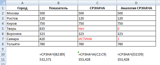
The younger brother of the AVERAGE function, everything is calculated exactly the same, but empty cells, text and FALSE/TRUE values ​​are taken into account. More precisely:

• I cells with text as a value, or empty (""), are counted as zero. If the expression should not contain text values, use the AVERAGE function.
• Cells with the value TRUE are counted as 1, and FALSE - respectively = 0.

An example can be seen in the picture:

Write comments with your questions!

In order to find the average value in Excel (no matter whether it is a numeric, text, percentage or other value), there are many functions. And each of them has its own characteristics and advantages. Indeed, in this task certain conditions may be set.

For example, the average values ​​of a series of numbers in Excel are calculated using statistical functions. You can also manually enter your own formula. Let's consider various options.

How to find the arithmetic mean of numbers?

To find the arithmetic mean, you need to add up all the numbers in the set and divide the sum by the quantity. For example, a student’s grades in computer science: 3, 4, 3, 5, 5. What is included in the quarter: 4. We found the arithmetic mean using the formula: =(3+4+3+5+5)/5.

How to quickly do this using Excel functions? Let's take for example a series of random numbers in a string:

Or: make the active cell and simply enter the formula manually: =AVERAGE(A1:A8).

Now let's see what else the AVERAGE function can do.

Let's find the arithmetic mean of the first two and last three numbers. Formula: =AVERAGE(A1:B1,F1:H1). Result:

Condition average

The condition for finding the arithmetic mean can be a numerical criterion or a text one. We will use the function: =AVERAGEIF().

Find the arithmetic mean of numbers that are greater than or equal to 10.

Function: =AVERAGEIF(A1:A8,">=10")

The third argument – ​​“Averaging range” – is omitted. First of all, it is not required. Secondly, the range analyzed by the program contains ONLY numeric values. The cells specified in the first argument will be searched according to the condition specified in the second argument.

Attention! The search criterion can be specified in the cell. And make a link to it in the formula.

Let's find the average value of the numbers using the text criterion. For example, the average sales of the product “tables”.

The function will look like this: =AVERAGEIF($A$2:$A$12,A7,$B$2:$B$12). Range – a column with product names. The search criterion is a link to a cell with the word “tables” (you can insert the word “tables” instead of link A7). Averaging range – those cells from which data will be taken to calculate the average value.

As a result of calculating the function, we obtain the following value:

Attention! For a text criterion (condition), the averaging range must be specified.

How to calculate the weighted average price in Excel?

How did we find out the weighted average price?

Formula: =SUMPRODUCT(C2:C12,B2:B12)/SUM(C2:C12).

Using the SUMPRODUCT formula, we find out the total revenue after selling the entire quantity of goods. And the SUM function sums up the quantity of goods. By dividing the total revenue from the sale of goods by the total number of units of goods, we found the weighted average price. This indicator takes into account the “weight” of each price. Its share in the total mass of values.

Standard deviation: formula in Excel

There are standard deviations for the general population and for the sample. In the first case, this is the root of the general variance. In the second, from the sample variance.

To calculate this statistical indicator, a dispersion formula is compiled. The root is extracted from it. But in Excel there is a ready-made function for finding the standard deviation.

The standard deviation is tied to the scale of the source data. This is not enough for a figurative representation of the variation of the analyzed range. To obtain the relative level of data scatter, the coefficient of variation is calculated:

standard deviation / arithmetic mean

The formula in Excel looks like this:

STDEV (range of values) / AVERAGE (range of values).

The coefficient of variation is calculated as a percentage. Therefore, we set the percentage format in the cell.

It gets lost in calculating the average.

Average meaning set of numbers is equal to the sum of numbers S divided by the number of these numbers. That is, it turns out that average meaning equals: 19/4 = 4.75.

Please note

If you need to find the geometric mean for just two numbers, then you don’t need an engineering calculator: you can extract the second root (square root) of any number using the most ordinary calculator.

Useful advice

Unlike the arithmetic mean, the geometric mean is not as strongly affected by large deviations and fluctuations between individual values ​​in the set of indicators under study.

Sources:

• Online calculator that calculates the geometric mean
• geometric mean formula

Average value is one of the characteristics of a set of numbers. Represents a number that cannot fall outside the range defined by the largest and smallest values ​​in that set of numbers. Average arithmetic value is the most commonly used type of average.

Instructions

Add up all the numbers in the set and divide them by the number of terms to get the arithmetic mean. Depending on the specific calculation conditions, it is sometimes easier to divide each of the numbers by the number of values ​​in the set and sum the result.

Use, for example, included in the Windows OS, if it is not possible to calculate the arithmetic average in your head. You can open it using the program launch dialog. To do this, press the hot keys WIN + R or click the Start button and select the Run command from the main menu. Then type calc in the input field and press Enter or click the OK button. The same can be done through the main menu - open it, go to the “All programs” section and in the “Standard” section and select the “Calculator” line.

Enter all the numbers in the set sequentially by pressing the Plus key after each of them (except the last one) or clicking the corresponding button in the calculator interface. You can also enter numbers either from the keyboard or by clicking the corresponding interface buttons.

Press the slash key or click this in the calculator interface after entering the last set value and type the number of numbers in the sequence. Then press the equal sign and the calculator will calculate and display the arithmetic mean.

You can use the Microsoft Excel spreadsheet editor for the same purpose. In this case, launch the editor and enter all the values ​​of the sequence of numbers into the adjacent cells. If, after entering each number, you press Enter or the down or right arrow key, the editor itself will move the input focus to the adjacent cell.

Click the cell next to the last number entered if you don't want to just see the average. Expand the Greek sigma (Σ) drop-down menu for the Edit commands on the Home tab. Select the line " Average" and the editor will insert the desired formula for calculating the arithmetic mean into the selected cell. Press the Enter key and the value will be calculated.

The arithmetic mean is one of the measures of central tendency, widely used in mathematics and statistical calculations. Finding the arithmetic average for several values ​​is very simple, but each task has its own nuances, which are simply necessary to know in order to perform correct calculations.

What is an arithmetic mean

How to find the arithmetic mean

Features of working with negative numbers

1. Finding the general arithmetic average using the standard method;
2. Finding the arithmetic mean of negative numbers.
3. Calculation of the arithmetic mean of positive numbers.

The responses for each action are written separated by commas.

Natural and decimal fractions

When working with natural fractions, they should be reduced to a common denominator, which is multiplied by the number of numbers in the array. The numerator of the answer will be the sum of the given numerators of the original fractional elements.

• Engineering calculator.

Instructions

Keep in mind that in general, the geometric mean of numbers is found by multiplying these numbers and taking the root of the power from them, which corresponds to the number of numbers. For example, if you need to find the geometric mean of five numbers, then you will need to extract the root of the power from the product.

To find the geometric mean of two numbers, use the basic rule. Find their product, then take the square root of it, since the number is two, which corresponds to the power of the root. For example, in order to find the geometric mean of the numbers 16 and 4, find their product 16 4 = 64. From the resulting number, extract the square root √64=8. This will be the desired value. Please note that the arithmetic mean of these two numbers is greater than and equal to 10. If the entire root is not extracted, round the result to the desired order.

To find the geometric mean of more than two numbers, also use the basic rule. To do this, find the product of all numbers for which you need to find the geometric mean. From the resulting product, extract the root of the power equal to the number of numbers. For example, to find the geometric mean of the numbers 2, 4, and 64, find their product. 2 4 64=512. Since you need to find the result of the geometric mean of three numbers, take the third root of the product. It is difficult to do this verbally, so use an engineering calculator. For this purpose it has a button "x^y". Dial the number 512, press the "x^y" button, then dial the number 3 and press the "1/x" button, to find the value of 1/3, press the "=" button. We get the result of raising 512 to the power of 1/3, which corresponds to the third root. Get 512^1/3=8. This is the geometric mean of the numbers 2.4 and 64.

Using an engineering calculator, you can find the geometric mean in another way. Find the log button on your keyboard. After that, take the logarithm for each of the numbers, find their sum and divide it by the number of numbers. Take the antilogarithm from the resulting number. This will be the geometric mean of the numbers. For example, in order to find the geometric mean of the same numbers 2, 4 and 64, perform a set of operations on the calculator. Dial the number 2, then press the log button, press the "+" button, dial the number 4 and press log and "+" again, dial 64, press log and "=". The result will be a number equal to the sum of the decimal logarithms of the numbers 2, 4 and 64. Divide the resulting number by 3, since this is the number of numbers for which the geometric mean is sought. From the result, take the antilogarithm by switching the case button and use the same log key. The result will be the number 8, this is the desired geometric mean.

Good afternoon, dear theorists and practitioners of statistical data analysis.

In this article we will continue the conversation we once started about averages. This time we will move from theory to practical calculations. The topic is vast even theoretically. If you add practical nuances, it becomes even more interesting. Let me remind you that some questions about averages are discussed in articles on the essence of the average, its main purpose and the weighted average. The properties of the indicator and its behavior were also considered depending on the initial data: a small sample and the presence of anomalous values.

These articles should generally give a good idea of ​​the rules of calculation and the correct use of averages. But now it’s the 21st (twenty-first) century and manual counting is quite rare, which, unfortunately, does not have a positive effect on the mental abilities of citizens. Even calculators are not in fashion (including programmable and engineering ones), much less abacus and slide rules. In short, all kinds of statistical calculations are now done in a program such as the Excel spreadsheet processor. I already wrote something about Excel, but then I temporarily abandoned it. For now, I decided to pay more attention to theoretical issues of data analysis, so that when describing calculations, for example, in Excel, I could refer to basic knowledge of statistics. In general, today we will talk about how to calculate the average in Excel. Let me just clarify that we are talking about the arithmetic average (yes, there are other average values, but they are used much less frequently).

The arithmetic mean is one of the most commonly used statistical indicators. The analyst simply needs to be able to use Excel to calculate it, as well as to calculate other indicators. And in general, an analyst without mastery of Excel is an impostor, not an analyst.

An inquisitive reader may ask: what is there to count? – I wrote the formula and that’s it. This is, of course, true, Excel calculates using a formula, but the type of formula and the result strongly depend on the source data. And the source data can be very different, including dynamic, that is, changeable. Therefore, adjusting one formula so that it is suitable for all occasions is not such a trivial matter.

Let's start with simple ones, then move on to more complex and, accordingly, more interesting ones. The simplest thing is if you need to draw a table with data, and below, in the final line, show the average value. To do this, if you are a “blonde”, you can use the summation of individual cells using a plus sign (after putting it in brackets) and then dividing by the number of these cells. If you are a “brunette”, then instead of separately marking cells with a “+” sign, you can use the summation formula SUM() and then divide by the number of values. However, more advanced Excel users know that there is a ready-made formula - AVERAGE(). The range of initial data from which the average value is calculated is indicated in parentheses, which is convenient to do with a mouse (computer).

Formula AVERAGE

The Excel statistical function AVERAGE is used quite often. It looks something like this.

This formula has a remarkable property that gives it value and sets it apart from manual summation and division by the number of values. If the range by which the formula is calculated contains empty cells (not zero, but empty), then this value is ignored and excluded from the calculation. Thus, if there is missing data for some observations, the average value will not be underestimated (when summing, an empty cell is perceived by Excel as zero). This fact makes the AVERAGE formula a valuable tool in the analyst’s arsenal.

There are different ways to get to the formula. First, you need to select the cell in which the formula will appear. The formula itself can be entered manually in the formula bar, or you can use its presence on the taskbar - the “Home” tab, at the top right there is a pull-out button with the autosum icon Σ:

After calling the formula, in parentheses you will need to specify the range of data for which the average value will be calculated. This can be done with the mouse by pressing the left key and dragging across the desired range. If the data range is not continuous, then by holding down the Ctrl key on the keyboard, you can select the necessary places. Next, press “Enter”. This method is very convenient and is often used.

There is also a standard calling method for all functions. You need to press a button fx at the beginning of the line where functions (formulas) are written and thereby call the Function Wizard. Then, either using a search or simply using the list, select the AVERAGE function (you can pre-sort the entire list of functions by the “statistical” category).

After selecting the function, press “Enter” or “Ok” and then select the range or ranges. Click on “Enter” or “Ok” again. The calculation result will be reflected in the cell with the formula. It's simple.

Calculation of arithmetic weighted average in Excel

(module 111)

As you might guess, the AVERAGE formula can only calculate the simple arithmetic mean, that is, it adds everything up and divides it by the number of terms (minus the number of empty cells). However, you often have to deal with a weighted arithmetic average. There is no ready-made formula in Excel, at least I haven’t found one. Therefore, you will have to use several formulas here. There is no need to be scared, it is not much more difficult than using AVERAGE, except that you will need to make a couple of extra movements.

Let me remind you that the formula for the weighted arithmetic average assumes in the numerator the sum of the products of the values ​​of the analyzed indicator and the corresponding weights. There are different opportunities to get the required amount. Often an intermediate calculation is made in a separate column, in which the product of each value and its corresponding weight is calculated. Then the sum of these products is calculated. This gives the numerator of the weighted average formula. Then all this is divided by the sum of the weights, in the same or a separate cell. It looks something like this.

In general, the Excel developers clearly did not finalize this point. You have to dodge and calculate the weighted average in the “semi-automatic” mode. However, it is possible to reduce the number of calculations. There is a wonderful SUMPRODUCT function for this. Using this function, you can avoid the intermediate calculation in the adjacent column and calculate the numerator with one function. You can divide by the sum of the weights in the same cell by adding the formula manually, or in the next one.

As you can see, there are several options. In general, the same tasks in Excel can be solved in different ways, which makes the spreadsheet processor very flexible and practical.

Calculation of the arithmetic mean by condition

When calculating the average value, situations may arise when not all values ​​need to be included in the calculation, but only the necessary ones that satisfy certain conditions (for example, goods for individual product groups). There is a ready-made formula for this AVERAGEIF.

It happens that the average value needs to be calculated from filtered values. There is also such a possibility - the SUBTOTAL function. The formula selection parameter should be set to 1 (and not 9, as in the case of summation).

Excel offers quite a lot of options for calculating averages. I have only described the main and most popular methods. It is impossible to sort out all the existing options; there are millions of them. However, what is described above occurs in 90% of cases and is quite sufficient for successful use. The main thing here is to clearly understand what is being done and why. Excel does not analyze, but only helps to quickly make calculations. Behind any formulas there must be cold calculation and a sober understanding of the analysis being carried out.

That's probably all you need to know about calculating the arithmetic average in Excel first of all.

Below is a video about the AVERAGEIF function and calculating the weighted arithmetic average in Excel

In most cases, data is concentrated around some central point. Thus, to describe any set of data, it is enough to indicate the average value. Let us consider sequentially three numerical characteristics that are used to estimate the average value of the distribution: arithmetic mean, median and mode.

Arithmetic mean

The arithmetic mean (often called simply the mean) is the most common estimate of the mean of a distribution. It is the result of dividing the sum of all observed numerical values ​​by their number. For a sample consisting of numbers X 1, X 2, …, Xn, sample mean (denoted by ) equals = (X 1 + X 2 + … + Xn) / n, or

where is the sample mean, n- sample size, Xi– i-th element of the sample.

Download the note in or format, examples in format

Consider calculating the arithmetic average of the five-year average annual returns of 15 very high-risk mutual funds (Figure 1).

Rice. 1. Average annual returns of 15 very high-risk mutual funds

The sample mean is calculated as follows:

This is a good return, especially compared to the 3-4% return that bank or credit union depositors received over the same time period. If we sort the returns, it is easy to see that eight funds have returns above the average, and seven - below the average. The arithmetic mean acts as the equilibrium point, so that funds with low returns balance out funds with high returns. All elements of the sample are involved in calculating the average. None of the other estimates of the mean of a distribution have this property.

When should you calculate the arithmetic mean? Since the arithmetic mean depends on all elements in the sample, the presence of extreme values ​​significantly affects the result. In such situations, the arithmetic mean can distort the meaning of numerical data. Therefore, when describing a data set containing extreme values, it is necessary to indicate the median or the arithmetic mean and the median. For example, if we remove the RS Emerging Growth fund's returns from the sample, the sample average of the 14 funds' returns decreases by almost 1% to 5.19%.

Median

The median represents the middle value of an ordered array of numbers. If the array does not contain repeating numbers, then half of its elements will be less than, and half will be greater than, the median. If the sample contains extreme values, it is better to use the median rather than the arithmetic mean to estimate the mean. To calculate the median of a sample, it must first be ordered.

This formula is ambiguous. Its result depends on whether the number is even or odd n:

• If the sample contains an odd number of elements, the median is (n+1)/2-th element.
• If the sample contains an even number of elements, the median lies between the two middle elements of the sample and is equal to the arithmetic mean calculated over these two elements.

To calculate the median of a sample containing the returns of 15 very high-risk mutual funds, you first need to sort the raw data (Figure 2). Then the median will be opposite the number of the middle element of the sample; in our example No. 8. Excel has a special function =MEDIAN() that works with unordered arrays too.

Rice. 2. Median 15 funds

Thus, the median is 6.5. This means that the return on one half of the very high-risk funds does not exceed 6.5, and the return on the other half exceeds it. Note that the median of 6.5 is not much larger than the mean of 6.08.

If we remove the return of the RS Emerging Growth fund from the sample, then the median of the remaining 14 funds decreases to 6.2%, that is, not as significantly as the arithmetic mean (Figure 3).

Rice. 3. Median 14 funds

Fashion

The term was first coined by Pearson in 1894. Fashion is the number that occurs most often in a sample (the most fashionable). Fashion describes well, for example, the typical reaction of drivers to a traffic light signal to stop moving. A classic example of the use of fashion is the choice of shoe size or wallpaper color. If a distribution has several modes, then it is said to be multimodal or multimodal (has two or more “peaks”). The multimodality of the distribution provides important information about the nature of the variable being studied. For example, in sociological surveys, if a variable represents a preference or attitude towards something, then multimodality may mean that there are several distinctly different opinions. Multimodality also serves as an indicator that the sample is not homogeneous and the observations may be generated by two or more “overlapping” distributions. Unlike the arithmetic mean, outliers do not affect the mode. For continuously distributed random variables, such as the average annual return of mutual funds, the mode sometimes does not exist (or makes no sense) at all. Since these indicators can take on very different values, repeating values ​​are extremely rare.

Quartiles

Quartiles are the metrics most often used to evaluate the distribution of data when describing the properties of large numerical samples. While the median splits the ordered array in half (50% of the array's elements are less than the median and 50% are greater), quartiles split the ordered data set into four parts. The values ​​of Q 1 , median and Q 3 are the 25th, 50th and 75th percentiles, respectively. The first quartile Q 1 is a number that divides the sample into two parts: 25% of the elements are less than, and 75% are greater than, the first quartile.

The third quartile Q 3 is a number that also divides the sample into two parts: 75% of the elements are less than, and 25% are greater than, the third quartile.

To calculate quartiles in versions of Excel before 2007, use the =QUARTILE(array,part) function. Starting from Excel 2010, two functions are used:

• =QUARTILE.ON(array,part)
• =QUARTILE.EXC(array,part)

These two functions give slightly different values ​​(Figure 4). For example, when calculating the quartiles of a sample containing the average annual returns of 15 very high-risk mutual funds, Q 1 = 1.8 or –0.7 for QUARTILE.IN and QUARTILE.EX, respectively. By the way, the QUARTILE function, previously used, corresponds to the modern QUARTILE.ON function. To calculate quartiles in Excel using the above formulas, the data array does not need to be ordered.

Rice. 4. Calculating quartiles in Excel

Let us emphasize again. Excel can calculate quartiles for a univariate discrete series, containing the values ​​of a random variable. The calculation of quartiles for a frequency-based distribution is given below in the section.

Geometric mean

Unlike the arithmetic mean, the geometric mean allows you to estimate the degree of change in a variable over time. The geometric mean is the root n th degree from the work n quantities (in Excel the =SRGEOM function is used):

G= (X 1 * X 2 * … * X n) 1/n

A similar parameter - the geometric mean value of the rate of profit - is determined by the formula:

G = [(1 + R 1) * (1 + R 2) * … * (1 + R n)] 1/n – 1,

Where R i– rate of profit for i th time period.

For example, suppose the initial investment is $100,000. By the end of the first year, it falls to $50,000, and by the end of the second year it recovers to the initial level of $100,000. The rate of return on this investment over a two-year period equals 0, since the initial and final amounts of funds are equal to each other. However, the arithmetic average of the annual profit rates is = (–0.5 + 1) / 2 = 0.25 or 25%, since the profit rate in the first year R 1 = (50,000 – 100,000) / 100,000 = –0.5 , and in the second R 2 = (100,000 – 50,000) / 50,000 = 1. At the same time, the geometric mean value of the rate of profit for two years is equal to: G = [(1–0.5) * (1+1 )] 1/2 – 1 = ½ – 1 = 1 – 1 = 0. Thus, the geometric mean more accurately reflects the change (more precisely, the absence of changes) in the volume of investments over a two-year period than the arithmetic mean.

Interesting facts. Firstly, the geometric mean will always be less than the arithmetic mean of the same numbers. Except for the case when all the numbers taken are equal to each other. Secondly, by considering the properties of a right triangle, you can understand why the mean is called geometric. The height of a right triangle, lowered to the hypotenuse, is the average proportional between the projections of the legs onto the hypotenuse, and each leg is the average proportional between the hypotenuse and its projection onto the hypotenuse (Fig. 5). This gives a geometric way to construct the geometric mean of two (lengths) segments: you need to construct a circle on the sum of these two segments as a diameter, then the height restored from the point of their connection to the intersection with the circle will give the desired value:

Rice. 5. Geometric nature of the geometric mean (figure from Wikipedia)

The second important property of numerical data is their variation, characterizing the degree of data dispersion. Two different samples may differ in both means and variances. However, as shown in Fig. 6 and 7, two samples may have the same variations but different means, or the same means and completely different variations. The data that corresponds to polygon B in Fig. 7, change much less than the data on which polygon A was constructed.

Rice. 6. Two symmetrical bell-shaped distributions with the same spread and different mean values

Rice. 7. Two symmetrical bell-shaped distributions with the same mean values ​​and different spreads

There are five estimates of data variation:

• scope,
• interquartile range,
• dispersion,
• standard deviation,
• coefficient of variation.

Scope

The range is the difference between the largest and smallest elements of the sample:

Range = XMax – XMin

The range of a sample containing the average annual returns of 15 very high-risk mutual funds can be calculated using the ordered array (see Figure 4): Range = 18.5 – (–6.1) = 24.6. This means that the difference between the highest and lowest average annual returns of very high-risk funds is 24.6%.

Range measures the overall spread of data. Although sample range is a very simple estimate of the overall spread of the data, its weakness is that it does not take into account exactly how the data are distributed between the minimum and maximum elements. This effect is clearly visible in Fig. 8, which illustrates samples having the same range. Scale B demonstrates that if a sample contains at least one extreme value, the sample range is a very imprecise estimate of the spread of the data.

Rice. 8. Comparison of three samples with the same range; the triangle symbolizes the support of the scale, and its location corresponds to the sample mean

Interquartile range

The interquartile, or average, range is the difference between the third and first quartiles of the sample:

Interquartile range = Q 3 – Q 1

This value allows us to estimate the scatter of 50% of the elements and not take into account the influence of extreme elements. The interquartile range of a sample containing the average annual returns of 15 very high-risk mutual funds can be calculated using the data in Fig. 4 (for example, for the QUARTILE.EXC function): Interquartile range = 9.8 – (–0.7) = 10.5. The interval bounded by the numbers 9.8 and -0.7 is often called the middle half.

It should be noted that the values ​​of Q 1 and Q 3 , and hence the interquartile range, do not depend on the presence of outliers, since their calculation does not take into account any value that would be less than Q 1 or greater than Q 3 . Summary measures such as the median, first and third quartiles, and interquartile range that are not affected by outliers are called robust measures.

Although range and interquartile range provide estimates of the overall and average spread of a sample, respectively, neither of these estimates takes into account exactly how the data are distributed. Variance and standard deviation are devoid of this drawback. These indicators allow you to assess the degree to which data fluctuates around the average value. Sample variance is an approximation of the arithmetic mean calculated from the squares of the differences between each sample element and the sample mean. For a sample X 1, X 2, ... X n, the sample variance (denoted by the symbol S 2 is given by the following formula:

In general, sample variance is the sum of the squares of the differences between the sample elements and the sample mean, divided by a value equal to the sample size minus one:

Where - arithmetic mean, n- sample size, X i - i th selection element X. In Excel before version 2007, the function =VARP() was used to calculate the sample variance; since version 2010, the function =VARP.V() is used.

The most practical and widely accepted estimate of the spread of data is sample standard deviation. This indicator is denoted by the symbol S and is equal to the square root of the sample variance:

In Excel before version 2007, the function =STDEV.() was used to calculate the standard sample deviation; since version 2010, the function =STDEV.V() is used. To calculate these functions, the data array may be unordered.

Neither the sample variance nor the sample standard deviation can be negative. The only situation in which the indicators S 2 and S can be zero is if all elements of the sample are equal to each other. In this completely improbable case, the range and interquartile range are also zero.

Numerical data is inherently volatile. Any variable can take on many different values. For example, different mutual funds have different rates of return and loss. Due to the variability of numerical data, it is very important to study not only estimates of the mean, which are summary in nature, but also estimates of variance, which characterize the spread of the data.

Dispersion and standard deviation allow you to evaluate the spread of data around the average value, in other words, determine how many sample elements are less than the average and how many are greater. Dispersion has some valuable mathematical properties. However, its value is the square of the unit of measurement - square percent, square dollar, square inch, etc. Therefore, a natural measure of dispersion is the standard deviation, which is expressed in common units of income percentage, dollars, or inches.

Standard deviation allows you to estimate the amount of variation of sample elements around the average value. In almost all situations, the majority of observed values ​​lie within the range of plus or minus one standard deviation from the mean. Consequently, knowing the arithmetic mean of the sample elements and the standard sample deviation, it is possible to determine the interval to which the bulk of the data belongs.

The standard deviation of returns for the 15 very high-risk mutual funds is 6.6 (Figure 9). This means that the profitability of the bulk of funds differs from the average value by no more than 6.6% (i.e., it fluctuates in the range from –S= 6.2 – 6.6 = –0.4 to +S= 12.8). In fact, the five-year average annual return of 53.3% (8 out of 15) of the funds lies within this range.

Rice. 9. Sample standard deviation

Note that when summing the squared differences, sample items that are further away from the mean are weighted more heavily than items that are closer to the mean. This property is the main reason why the arithmetic mean is most often used to estimate the mean of a distribution.

Coefficient of variation

Unlike previous estimates of scatter, the coefficient of variation is a relative estimate. It is always measured as a percentage and not in the units of the original data. The coefficient of variation, denoted by the symbols CV, measures the dispersion of the data around the mean. The coefficient of variation is equal to the standard deviation divided by the arithmetic mean and multiplied by 100%:

Where S- standard sample deviation, - sample average.

The coefficient of variation allows you to compare two samples whose elements are expressed in different units of measurement. For example, the manager of a mail delivery service intends to renew his fleet of trucks. When loading packages, there are two restrictions to consider: the weight (in pounds) and the volume (in cubic feet) of each package. Suppose that in a sample containing 200 bags, the mean weight is 26.0 pounds, the standard deviation of weight is 3.9 pounds, the mean bag volume is 8.8 cubic feet, and the standard deviation of volume is 2.2 cubic feet. How to compare the variation in weight and volume of packages?

Since the units of measurement for weight and volume differ from each other, the manager must compare the relative spread of these quantities. The coefficient of variation of weight is CV W = 3.9 / 26.0 * 100% = 15%, and the coefficient of variation of volume is CV V = 2.2 / 8.8 * 100% = 25%. Thus, the relative variation in the volume of packets is much greater than the relative variation in their weight.

Distribution form

The third important property of a sample is the shape of its distribution. This distribution may be symmetrical or asymmetrical. To describe the shape of a distribution, it is necessary to calculate its mean and median. If the two are the same, the variable is considered symmetrically distributed. If the mean value of a variable is greater than the median, its distribution has a positive skewness (Fig. 10). If the median is greater than the mean, the distribution of the variable is negatively skewed. Positive skewness occurs when the mean increases to unusually high values. Negative skewness occurs when the mean decreases to unusually small values. A variable is symmetrically distributed if it does not take any extreme values ​​in either direction, so that large and small values ​​of the variable cancel each other out.

Rice. 10. Three types of distributions

Data shown on scale A are negatively skewed. This figure shows a long tail and a leftward skew caused by the presence of unusually small values. These extremely small values ​​shift the average value to the left, making it less than the median. The data shown on scale B is distributed symmetrically. The left and right halves of the distribution are mirror images of themselves. Large and small values ​​balance each other, and the mean and median are equal. The data shown on scale B is positively skewed. This figure shows a long tail and a skew to the right caused by the presence of unusually high values. These too large values ​​shift the mean to the right, making it larger than the median.

In Excel, descriptive statistics can be obtained using an add-in Analysis package. Go through the menu Data → Data Analysis, in the window that opens, select the line Descriptive Statistics and click Ok. In the window Descriptive Statistics be sure to indicate Input interval(Fig. 11). If you want to see descriptive statistics on the same sheet as the original data, select the radio button Output interval and specify the cell where the upper left corner of the displayed statistics should be placed (in our example, $C$1). If you want to output data to a new sheet or a new workbook, you just need to select the appropriate radio button. Check the box next to Summary statistics. If desired, you can also choose Difficulty levelkth smallest andkth largest.

If on deposit Data in the area Analysis you don't see the icon Data Analysis, you must first install the add-on Analysis package(see, for example,).

Rice. 11. Descriptive statistics of five-year average annual returns of funds with very high levels of risk, calculated using the add-in Data Analysis Excel programs

Excel calculates a number of statistics discussed above: mean, median, mode, standard deviation, variance, range ( interval), minimum, maximum and sample size ( check). Excel also calculates some statistics that are new to us: standard error, kurtosis, and skewness. Standard error equal to the standard deviation divided by the square root of the sample size. Asymmetry characterizes the deviation from the symmetry of the distribution and is a function that depends on the cube of the differences between the sample elements and the average value. Kurtosis is a measure of the relative concentration of data around the mean compared to the tails of the distribution and depends on the differences between the sample elements and the mean raised to the fourth power.

Calculating descriptive statistics for the population

The mean, spread, and shape of the distribution discussed above are characteristics determined from the sample. However, if the data set contains numerical measurements of the entire population, its parameters can be calculated. Such parameters include the expected value, dispersion and standard deviation of the population.

Expectation equal to the sum of all values ​​in the population divided by the size of the population:

Where µ - mathematical expectation, Xi- i th observation of the variable X, N- volume of the general population. In Excel, to calculate the mathematical expectation, the same function is used as for the arithmetic average: =AVERAGE().

Population variance equal to the sum of the squares of the differences between the elements of the general population and the mat. expectation divided by the size of the population:

Where σ 2– dispersion of the general population. In Excel prior to version 2007, the =VARP() function is used to calculate the population variance, starting with version 2010 =VARP().

Population standard deviation equal to the square root of the population variance:

In Excel prior to version 2007, the =STDEV() function is used to calculate the standard deviation of a population; since version 2010, =STDEV.Y(). Note that the formulas for the population variance and standard deviation are different from the formulas for calculating the sample variance and standard deviation. When calculating sample statistics S 2 And S the denominator of the fraction is n – 1, and when calculating parameters σ 2 And σ - volume of the general population N.

Rule of thumb

In most situations, a large proportion of observations are concentrated around the median, forming a cluster. In data sets with positive skewness, this cluster is located to the left (i.e., below) the mathematical expectation, and in sets with negative skewness, this cluster is located to the right (i.e., above) the mathematical expectation. For symmetric data, the mean and median are the same, and observations cluster around the mean, forming a bell-shaped distribution. If the distribution is not clearly skewed and the data is concentrated around a center of gravity, a rule of thumb that can be used to estimate variability is that if the data has a bell-shaped distribution, then approximately 68% of the observations are within one standard deviation of the expected value. approximately 95% of observations are no more than two standard deviations away from the mathematical expectation and 99.7% of observations are no more than three standard deviations away from the mathematical expectation.

Thus, the standard deviation, which is an estimate of the average variation around the expected value, helps to understand how observations are distributed and to identify outliers. The rule of thumb is that for bell-shaped distributions, only one value in twenty differs from the mathematical expectation by more than two standard deviations. Therefore, values ​​outside the interval µ ± 2σ, can be considered outliers. In addition, only three out of 1000 observations differ from the mathematical expectation by more than three standard deviations. Thus, values ​​outside the interval µ ± 3σ are almost always outliers. For distributions that are highly skewed or not bell-shaped, the Bienamay-Chebyshev rule of thumb can be applied.

More than a hundred years ago, mathematicians Bienamay and Chebyshev independently discovered the useful property of standard deviation. They found that for any data set, regardless of the shape of the distribution, the percentage of observations lying within a distance of k standard deviations from mathematical expectation, not less (1 – 1/ k 2)*100%.

For example, if k= 2, the Bienname-Chebyshev rule states that at least (1 – (1/2) 2) x 100% = 75% of the observations must lie in the interval µ ± 2σ. This rule is true for any k, exceeding one. The Bienamay-Chebyshev rule is very general and valid for distributions of any type. It specifies the minimum number of observations, the distance from which to the mathematical expectation does not exceed a specified value. However, if the distribution is bell-shaped, the rule of thumb more accurately estimates the concentration of data around the expected value.

Calculating Descriptive Statistics for a Frequency-Based Distribution

If the original data are not available, the frequency distribution becomes the only source of information. In such situations, it is possible to calculate approximate values ​​of quantitative indicators of the distribution, such as the arithmetic mean, standard deviation, and quartiles.

If sample data is represented as a frequency distribution, an approximation of the arithmetic mean can be calculated by assuming that all values ​​within each class are concentrated at the class midpoint:

Where - sample average, n- number of observations, or sample size, With- number of classes in the frequency distribution, m j- midpoint j th class, fj- frequency corresponding j-th class.

To calculate the standard deviation from a frequency distribution, it is also assumed that all values ​​within each class are concentrated at the class midpoint.

To understand how quartiles of a series are determined based on frequencies, consider the calculation of the lower quartile based on data for 2013 on the distribution of the Russian population by average per capita monetary income (Fig. 12).

Rice. 12. Share of the Russian population with average per capita cash income per month, rubles

To calculate the first quartile of an interval variation series, you can use the formula:

where Q1 is the value of the first quartile, xQ1 is the lower limit of the interval containing the first quartile (the interval is determined by the accumulated frequency that first exceeds 25%); i – interval value; Σf – sum of frequencies of the entire sample; probably always equal to 100%; SQ1–1 – accumulated frequency of the interval preceding the interval containing the lower quartile; fQ1 – frequency of the interval containing the lower quartile. The formula for the third quartile differs in that in all places you need to use Q3 instead of Q1, and substitute ¾ instead of ¼.

In our example (Fig. 12), the lower quartile is in the range 7000.1 – 10,000, the accumulated frequency of which is 26.4%. The lower limit of this interval is 7000 rubles, the value of the interval is 3000 rubles, the accumulated frequency of the interval preceding the interval containing the lower quartile is 13.4%, the frequency of the interval containing the lower quartile is 13.0%. Thus: Q1 = 7000 + 3000 * (¼ * 100 – 13.4) / 13 = 9677 rub.

Pitfalls Associated with Descriptive Statistics

In this post, we looked at how to describe a data set using various statistics that evaluate its mean, spread, and distribution. The next step is data analysis and interpretation. Until now, we have studied the objective properties of data, and now we move on to their subjective interpretation. The researcher faces two mistakes: an incorrectly chosen subject of analysis and an incorrect interpretation of the results.

The analysis of the returns of 15 very high-risk mutual funds is quite unbiased. He led to completely objective conclusions: all mutual funds have different returns, the spread of fund returns ranges from -6.1 to 18.5, and the average return is 6.08. The objectivity of data analysis is ensured by the correct choice of summary quantitative indicators of distribution. Several methods for estimating the mean and scatter of data were considered, and their advantages and disadvantages were indicated. How do you choose the right statistics to provide an objective and impartial analysis? If the data distribution is slightly skewed, should you choose the median rather than the mean? Which indicator more accurately characterizes the spread of data: standard deviation or range? Should we point out that the distribution is positively skewed?

On the other hand, data interpretation is a subjective process. Different people come to different conclusions when interpreting the same results. Everyone has their own point of view. Someone considers the total average annual returns of 15 funds with a very high level of risk to be good and is quite satisfied with the income received. Others may feel that these funds have too low returns. Thus, subjectivity should be compensated by honesty, neutrality and clarity of conclusions.

Ethical issues

Data analysis is inextricably linked to ethical issues. You should be critical of information disseminated by newspapers, radio, television and the Internet. Over time, you will learn to be skeptical not only of the results, but also of the goals, subject matter and objectivity of the research. The famous British politician Benjamin Disraeli said it best: “There are three kinds of lies: lies, damned lies and statistics.”

As noted in the note, ethical issues arise when choosing the results that should be presented in the report. Both positive and negative results should be published. In addition, when making a report or written report, the results must be presented honestly, neutrally and objectively. There is a distinction to be made between unsuccessful and dishonest presentations. To do this, it is necessary to determine what the speaker's intentions were. Sometimes the speaker omits important information out of ignorance, and sometimes it is deliberate (for example, if he uses the arithmetic mean to estimate the average of clearly skewed data in order to obtain the desired result). It is also dishonest to suppress results that do not correspond to the researcher's point of view.

Materials from the book Levin et al. Statistics for Managers are used. – M.: Williams, 2004. – p. 178–209

The QUARTILE function has been retained for compatibility with earlier versions of Excel.