Matrix operations. Square matrix multiplication

Matrix dimension is a rectangular table consisting of elements located in m lines and n columns.

Matrix elements (first index i− line number, second index j− column number) can be numbers, functions, etc. Matrices are denoted by capital letters of the Latin alphabet.

The matrix is ​​called square, if it has the same number of rows as the number of columns ( m = n). In this case the number n is called the order of the matrix, and the matrix itself is called a matrix n-th order.

Elements with the same indexes form main diagonal square matrix, and the elements (i.e. having a sum of indices equal to n+1) − side diagonal.

Single matrix is a square matrix, all elements of the main diagonal of which are equal to 1, and the remaining elements are equal to 0. It is denoted by the letter E.

Zero matrix− is a matrix, all elements of which are equal to 0. A zero matrix can be of any size.

To the number linear operations on matrices include:

1) matrix addition;

2) multiplying matrices by number.

The matrix addition operation is defined only for matrices of the same dimension.

The sum of two matrices A And IN called a matrix WITH, all elements of which are equal to the sums of the corresponding matrix elements A And IN:

.

Matrix product A per number k called a matrix IN, all elements of which are equal to the corresponding elements of this matrix A, multiplied by the number k:

Operation matrix multiplication is introduced for matrices that satisfy the condition: the number of columns of the first matrix is ​​equal to the number of rows of the second.

Matrix product A dimensions to the matrix IN dimension is called a matrix WITH dimensions, element i-th line and j the th column of which is equal to the sum of the products of the elements i th row of the matrix A to the corresponding elements j th matrix column IN:

The product of matrices (unlike the product of real numbers) does not obey the commutative law, i.e. in general case A IN IN A.

1.2. Determinants. Properties of determinants

The concept of a determinant is introduced only for square matrices.

The determinant of a 2nd order matrix is ​​a number calculated according to the following rule

.

Determinant of a 3rd order matrix is a number calculated according to the following rule:

The first of the terms with the “+” sign is the product of the elements located on the main diagonal of the matrix (). The remaining two contain elements located at the vertices of triangles with the base parallel to the main diagonal (i). The “-” sign includes the products of the elements of the secondary diagonal () and the elements forming triangles with bases parallel to this diagonal (and).

This rule for calculating the 3rd order determinant is called the triangle rule (or Sarrus' rule).

Properties of determinants Let's look at the example of 3rd order determinants.

1. When replacing all rows of the determinant with columns with the same numbers as the rows, the determinant does not change its value, i.e. rows and columns of the determinant are equal

.

2. When two rows (columns) are rearranged, the determinant changes its sign.

3. If all elements of a certain row (column) are zeros, then the determinant is 0.

4. The common factor of all elements of a row (column) can be taken beyond the sign of the determinant.

5. The determinant containing two identical rows (columns) is equal to 0.

6. A determinant containing two proportional rows (columns) is equal to zero.

7. If each element of a certain column (row) of a determinant represents the sum of two terms, then the determinant is equal to the sum of two determinants, one of which contains the first terms in the same column (row), and the other contains the second. The remaining elements of both determinants are the same. So,

.

8. The determinant will not change if the corresponding elements of another column (row) are added to the elements of any of its columns (rows), multiplied by the same number.

Matrix addition:

Subtraction and addition of matrices reduces to the corresponding operations on their elements. Matrix addition operation entered only for matrices the same size, i.e. for matrices, in which the number of rows and columns is respectively equal. Sum of matrices A and B are called matrix C, whose elements are equal to the sum of the corresponding elements. C = A + B c ij = a ij + b ij Defined similarly matrix difference.

Multiplying a matrix by a number:

Matrix multiplication (division) operation of any size by an arbitrary number is reduced to multiplying (dividing) each element matrices for this number. Matrix product And the number k is called matrix B, such that

b ij = k × a ij . B = k × A b ij = k × a ij . Matrix- A = (-1) × A is called the opposite matrix A.

Properties of adding matrices and multiplying a matrix by a number:

Matrix addition operations And matrix multiplication on a number have the following properties: 1. A + B = B + A; 2. A + (B + C) = (A + B) + C; 3. A + 0 = A; 4. A - A = 0; 5. 1 × A = A; 6. α × (A + B) = αA + αB; 7. (α + β) × A = αA + βA; 8. α × (βA) = (αβ) × A; , where A, B and C are matrices, α and β are numbers.

Matrix multiplication (Matrix product):

Operation of multiplying two matrices is entered only for the case when the number of columns of the first matrices equal to the number of lines of the second matrices. Matrix product And m×n on matrix In n×p, called matrix With m×p such that with ik = a i1 × b 1k + a i2 × b 2k + ... + a in × b nk , i.e., the sum of the products of the elements of the i-th row is found matrices And to the corresponding elements of the jth column matrices B. If matrices A and B are squares of the same size, then the products AB and BA always exist. It is easy to show that A × E = E × A = A, where A is square matrix, E - unit matrix the same size.

Properties of matrix multiplication:

Matrix multiplication not commutative, i.e. AB ≠ BA even if both products are defined. However, if for any matrices the relationship AB=BA is satisfied, then such matrices are called commutative. The most typical example is a single matrix, which commutes with any other matrix the same size. Only square ones can be permutable matrices of the same order. A × E = E × A = A

Matrix multiplication has the following properties: 1. A × (B × C) = (A × B) × C; 2. A × (B + C) = AB + AC; 3. (A + B) × C = AC + BC; 4. α × (AB) = (αA) × B; 5. A × 0 = 0; 0 × A = 0; 6. (AB) T = B T A T; 7. (ABC) T = C T V T A T; 8. (A + B) T = A T + B T;

2. Determinants of the 2nd and 3rd orders. Properties of determinants.

Matrix determinant second order, or determinant second order is a number that is calculated by the formula:

Matrix determinant third order, or determinant third order is a number that is calculated by the formula:

This number represents an algebraic sum consisting of six terms. Each term contains exactly one element from each row and each column matrices. Each term consists of the product of three factors.

Signs with which members determinant of the matrix included in the formula finding the determinant of the matrix third order can be determined using the given scheme, which is called the rule of triangles or Sarrus's rule. The first three terms are taken with a plus sign and determined from the left figure, and the next three terms are taken with a minus sign and determined from the right figure.

Determine the number of terms to find determinant of the matrix, in an algebraic sum, you can calculate the factorial: 2! = 1 × 2 = 2 3! = 1 × 2 × 3 = 6

Properties of matrix determinants

Properties of matrix determinants:

Property #1:

Matrix determinant will not change if its rows are replaced with columns, each row with a column with the same number, and vice versa (Transposition). |A| = |A| T

Consequence:

Columns and Rows determinant of the matrix are equal, therefore, the properties inherent in rows are also fulfilled for columns.

Property #2:

When rearranging 2 rows or columns matrix determinant will change the sign to the opposite one, maintaining the absolute value, i.e.:

Property #3:

Matrix determinant having two identical rows is equal to zero.

Property #4:

Common factor of elements of any series determinant of the matrix can be taken as a sign determinant.

Corollaries from properties No. 3 and No. 4:

If all elements of a certain series (row or column) are proportional to the corresponding elements of a parallel series, then such matrix determinant equal to zero.

Property #5:

determinant of the matrix are equal to zero, then matrix determinant equal to zero.

Property #6:

If all elements of a row or column determinant presented as a sum of 2 terms, then determinant matrices can be represented as the sum of 2 determinants according to the formula:

Property #7:

If to any row (or column) determinant add the corresponding elements of another row (or column), multiplied by the same number, then matrix determinant will not change its value.

Example of using properties for calculation determinant of the matrix:

So, in the previous lesson we looked at the rules for adding and subtracting matrices. These are such simple operations that most students understand them literally right off the bat.

However, you rejoice early. The freebie is over - let's move on to multiplication. I’ll warn you right away: multiplying two matrices is not at all multiplying numbers located in cells with the same coordinates, as you might think. Everything is much more fun here. And we will have to start with preliminary definitions.

Matched matrices

One of the most important characteristics of a matrix is ​​its size. We've already talked about this a hundred times: the notation $A=\left[ m\times n \right]$ means that the matrix has exactly $m$ rows and $n$ columns. We have also already discussed how not to confuse rows with columns. Something else is important now.

Definition. Matrices of the form $A=\left[ m\times n \right]$ and $B=\left[ n\times k \right]$, in which the number of columns in the first matrix coincides with the number of rows in the second, are called consistent.

Once again: the number of columns in the first matrix is ​​equal to the number of rows in the second! From here we get two conclusions at once:

1. The order of the matrices is important to us. For example, the matrices $A=\left[ 3\times 2 \right]$ and $B=\left[ 2\times 5 \right]$ are consistent (2 columns in the first matrix and 2 rows in the second), but vice versa — matrices $B=\left[ 2\times 5 \right]$ and $A=\left[ 3\times 2 \right]$ are no longer consistent (5 columns in the first matrix are not 3 rows in the second ).
2. Consistency can be easily checked by writing down all the dimensions one after another. Using the example from the previous paragraph: “3 2 2 5” - there are identical numbers in the middle, so the matrices are consistent. But “2 5 3 2” are not consistent, since there are different numbers in the middle.

In addition, Captain Obviousness seems to hint that square matrices of the same size $\left[ n\times n \right]$ are always consistent.

In mathematics, when the order of listing objects is important (for example, in the definition discussed above, the order of matrices is important), we often talk about ordered pairs. We met them back in school: I think it’s a no brainer that the coordinates $\left(1;0 \right)$ and $\left(0;1 \right)$ define different points on the plane.

So: coordinates are also ordered pairs that are made up of numbers. But nothing prevents you from making such a pair from matrices. Then we can say: “An ordered pair of matrices $\left(A;B \right)$ is consistent if the number of columns in the first matrix matches the number of rows in the second.”

So what?

Definition of multiplication

Consider two consistent matrices: $A=\left[ m\times n \right]$ and $B=\left[ n\times k \right]$. And we define the multiplication operation for them.

Definition. The product of two matched matrices $A=\left[ m\times n \right]$ and $B=\left[ n\times k \right]$ is the new matrix $C=\left[ m\times k \right] $, the elements of which are calculated using the formula:

\[\begin(align) & ((c)_(i;j))=((a)_(i;1))\cdot ((b)_(1;j))+((a)_ (i;2))\cdot ((b)_(2;j))+\ldots +((a)_(i;n))\cdot ((b)_(n;j))= \\ & =\sum\limits_(t=1)^(n)(((a)_(i;t))\cdot ((b)_(t;j))) \end(align)\]

Such a product is denoted in the standard way: $C=A\cdot B$.

Those who see this definition for the first time immediately have two questions:

1. What kind of fierce game is this?
2. Why is it so difficult?

Well, first things first. Let's start with the first question. What do all these indices mean? And how not to make mistakes when working with real matrices?

First of all, we note that the long line for calculating $((c)_(i;j))$ (I specially put a semicolon between the indices so as not to get confused, but there is no need to put them at all - I myself got tired of typing the formula in the definition) actually comes down to a simple rule:

1. Take the $i$th row in the first matrix;
2. Take the $j$th column in the second matrix;
3. We get two sequences of numbers. We multiply the elements of these sequences with the same numbers, and then add the resulting products.

This process is easy to understand from the picture:

Once again: we fix row $i$ in the first matrix, column $j$ in the second matrix, multiply elements with the same numbers, and then add the resulting products - we get $((c)_(ij))$. And so on for all $1\le i\le m$ and $1\le j\le k$. Those. There will be $m\times k$ of such “perversions” in total.

In fact, we have already encountered matrix multiplication in the school curriculum, only in a greatly reduced form. Let the vectors be given:

\[\begin(align) & \vec(a)=\left(((x)_(a));((y)_(a));((z)_(a)) \right); \\ & \overrightarrow(b)=\left(((x)_(b));((y)_(b));((z)_(b)) \right). \\ \end(align)\]

Then their scalar product will be exactly the sum of pairwise products:

\[\overrightarrow(a)\times \overrightarrow(b)=((x)_(a))\cdot ((x)_(b))+((y)_(a))\cdot ((y )_(b))+((z)_(a))\cdot ((z)_(b))\]

Basically, back when the trees were greener and the skies were brighter, we simply multiplied the row vector $\overrightarrow(a)$ by the column vector $\overrightarrow(b)$.

Nothing has changed today. It’s just that now there are more of these row and column vectors.

But enough theory! Let's look at real examples. And let's start with the simplest case - square matrices.

Square matrix multiplication

Task 1. Do the multiplication:

\[\left[ \begin(array)(*(35)(r)) 1 & 2 \\ -3 & 4 \\\end(array) \right]\cdot \left[ \begin(array)(* (35)(r)) -2 & 4 \\ 3 & 1 \\\end(array) \right]\]

Solution. So, we have two matrices: $A=\left[ 2\times 2 \right]$ and $B=\left[ 2\times 2 \right]$. It is clear that they are consistent (square matrices of the same size are always consistent). Therefore, we perform the multiplication:

\[\begin(align) & \left[ \begin(array)(*(35)(r)) 1 & 2 \\ -3 & 4 \\\end(array) \right]\cdot \left[ \ begin(array)(*(35)(r)) -2 & 4 \\ 3 & 1 \\\end(array) \right]=\left[ \begin(array)(*(35)(r)) 1\cdot \left(-2 \right)+2\cdot 3 & 1\cdot 4+2\cdot 1 \\ -3\cdot \left(-2 \right)+4\cdot 3 & -3\cdot 4+4\cdot 1 \\\end(array) \right]= \\ & =\left[ \begin(array)(*(35)(r)) 4 & 6 \\ 18 & -8 \\\ end(array)\right]. \end(align)\]

That's it!

Answer: $\left[ \begin(array)(*(35)(r))4 & 6 \\ 18 & -8 \\\end(array) \right]$.

Task 2. Do the multiplication:

\[\left[ \begin(matrix) 1 & 3 \\ 2 & 6 \\\end(matrix) \right]\cdot \left[ \begin(array)(*(35)(r))9 & 6 \\ -3 & -2 \\\end(array) \right]\]

Solution. Again, consistent matrices, so we perform the following actions:\[\]

\[\begin(align) & \left[ \begin(matrix) 1 & 3 \\ 2 & 6 \\\end(matrix) \right]\cdot \left[ \begin(array)(*(35)() r)) 9 & 6 \\ -3 & -2 \\\end(array) \right]=\left[ \begin(array)(*(35)(r)) 1\cdot 9+3\cdot \ left(-3 \right) & 1\cdot 6+3\cdot \left(-2 \right) \\ 2\cdot 9+6\cdot \left(-3 \right) & 2\cdot 6+6\ cdot \left(-2 \right) \\\end(array) \right]= \\ & =\left[ \begin(matrix) 0 & 0 \\ 0 & 0 \\\end(matrix) \right] . \end(align)\]

As you can see, the result is a matrix filled with zeros

Answer: $\left[ \begin(matrix) 0 & 0 \\ 0 & 0 \\\end(matrix) \right]$.

From the above examples it is obvious that matrix multiplication is not such a complicated operation. At least for 2 by 2 square matrices.

In the process of calculations, we compiled an intermediate matrix, where we directly described which numbers are included in a particular cell. This is exactly what you should do when solving real problems.

Basic properties of the matrix product

In a nutshell. Matrix multiplication:

1. Non-commutative: $A\cdot B\ne B\cdot A$ in the general case. There are, of course, special matrices for which the equality $A\cdot B=B\cdot A$ (for example, if $B=E$ is the identity matrix), but in the vast majority of cases this does not work;
2. Associatively: $\left(A\cdot B \right)\cdot C=A\cdot \left(B\cdot C \right)$. There are no options here: adjacent matrices can be multiplied without worrying about what is to the left and to the right of these two matrices.
3. Distributively: $A\cdot \left(B+C \right)=A\cdot B+A\cdot C$ and $\left(A+B \right)\cdot C=A\cdot C+B\cdot C $ (due to the non-commutativity of the product, it is necessary to separately specify right and left distributivity.

And now - everything is the same, but in more detail.

Matrix multiplication is in many ways similar to classical number multiplication. But there are differences, the most important of which is that Matrix multiplication is, generally speaking, non-commutative.

Let's look again at the matrices from Problem 1. We already know their direct product:

\[\left[ \begin(array)(*(35)(r)) 1 & 2 \\ -3 & 4 \\\end(array) \right]\cdot \left[ \begin(array)(* (35)(r)) -2 & 4 \\ 3 & 1 \\\end(array) \right]=\left[ \begin(array)(*(35)(r))4 & 6 \\ 18 & -8 \\\end(array) \right]\]

But if we swap the matrices, we get a completely different result:

\[\left[ \begin(array)(*(35)(r)) -2 & 4 \\ 3 & 1 \\\end(array) \right]\cdot \left[ \begin(array)(* (35)(r)) 1 & 2 \\ -3 & 4 \\\end(array) \right]=\left[ \begin(matrix) -14 & 4 \\ 0 & 10 \\\end(matrix )\right]\]

It turns out that $A\cdot B\ne B\cdot A$. In addition, the multiplication operation is only defined for the consistent matrices $A=\left[ m\times n \right]$ and $B=\left[ n\times k \right]$, but no one has guaranteed that they will remain consistent. if they are swapped. For example, the matrices $\left[ 2\times 3 \right]$ and $\left[ 3\times 5 \right]$ are quite consistent in the specified order, but the same matrices $\left[ 3\times 5 \right] $ and $\left[ 2\times 3 \right]$ written in reverse order are no longer consistent. Sad.:(

Among square matrices of a given size $n$ there will always be those that give the same result both when multiplied in direct and in reverse order. How to describe all such matrices (and how many there are in general) is a topic for a separate lesson. We won't talk about that today. :)

However, matrix multiplication is associative:

\[\left(A\cdot B \right)\cdot C=A\cdot \left(B\cdot C \right)\]

Therefore, when you need to multiply several matrices in a row at once, it is not at all necessary to do it straight away: it is quite possible that some adjacent matrices, when multiplied, give an interesting result. For example, a zero matrix, as in Problem 2 discussed above.

In real problems, one most often has to multiply square matrices of size $\left[ n\times n \right]$. The set of all such matrices is denoted by $((M)^(n))$ (i.e., the entries $A=\left[ n\times n \right]$ and \ mean the same thing), and it will necessarily contain matrix $E$, which is called the identity matrix.

Definition. An identity matrix of size $n$ is a matrix $E$ such that for any square matrix $A=\left[ n\times n \right]$ the equality holds:

Such a matrix always looks the same: there are ones on its main diagonal, and zeros in all other cells.

\[\begin(align) & A\cdot \left(B+C \right)=A\cdot B+A\cdot C; \\ & \left(A+B \right)\cdot C=A\cdot C+B\cdot C. \\ \end(align)\]

In other words, if you need to multiply one matrix by the sum of two others, you can multiply it by each of these “other two” and then add the results. In practice, we usually have to perform the opposite operation: we notice the same matrix, take it out of brackets, perform addition and thereby simplify our life. :)

Note: to describe distributivity, we had to write two formulas: where the sum is in the second factor and where the sum is in the first. This happens precisely because matrix multiplication is non-commutative (and in general, in non-commutative algebra there are a lot of fun things that don’t even come to mind when working with ordinary numbers). And if, for example, you need to write down this property in an exam, then be sure to write both formulas, otherwise the teacher may get a little angry.

Okay, these were all fairy tales about square matrices. What about rectangular ones?

The case of rectangular matrices

But nothing - everything is the same as with square ones.

Task 3. Do the multiplication:

\[\left[ \begin(matrix) \begin(matrix) 5 \\ 2 \\ 3 \\\end(matrix) & \begin(matrix) 4 \\ 5 \\ 1 \\\end(matrix) \ \\end(matrix) \right]\cdot \left[ \begin(array)(*(35)(r)) -2 & 5 \\ 3 & 4 \\\end(array) \right]\]

Solution. We have two matrices: $A=\left[ 3\times 2 \right]$ and $B=\left[ 2\times 2 \right]$. Let's write down the numbers indicating the sizes in a row:

As you can see, the central two numbers coincide. This means that the matrices are consistent and can be multiplied. Moreover, at the output we get the matrix $C=\left[ 3\times 2 \right]$:

\[\begin(align) & \left[ \begin(matrix) \begin(matrix) 5 \\ 2 \\ 3 \\\end(matrix) & \begin(matrix) 4 \\ 5 \\ 1 \\ \end(matrix) \\\end(matrix) \right]\cdot \left[ \begin(array)(*(35)(r)) -2 & 5 \\ 3 & 4 \\\end(array) \right]=\left[ \begin(array)(*(35)(r)) 5\cdot \left(-2 \right)+4\cdot 3 & 5\cdot 5+4\cdot 4 \\ 2 \cdot \left(-2 \right)+5\cdot 3 & 2\cdot 5+5\cdot 4 \\ 3\cdot \left(-2 \right)+1\cdot 3 & 3\cdot 5+1 \cdot 4 \\\end(array) \right]= \\ & =\left[ \begin(array)(*(35)(r)) 2 & 41 \\ 11 & 30 \\ -3 & 19 \ \\end(array) \right]. \end(align)\]

Everything is clear: the final matrix has 3 rows and 2 columns. Quite $=\left[ 3\times 2 \right]$.

Answer: $\left[ \begin(array)(*(35)(r)) \begin(array)(*(35)(r)) 2 \\ 11 \\ -3 \\\end(array) & \begin(matrix) 41 \\ 30 \\ 19 \\\end(matrix) \\\end(array) \right]$.

Now let's look at one of the best training tasks for those who are just starting to work with matrices. In it you need not just multiply some two tablets, but first determine: is such multiplication permissible?

Problem 4. Find all possible pairwise products of matrices:

\\]; $B=\left[ \begin(matrix) \begin(matrix) 0 \\ 2 \\ 0 \\ 4 \\\end(matrix) & \begin(matrix) 1 \\ 0 \\ 3 \\ 0 \ \\end(matrix) \\\end(matrix) \right]$; $C=\left[ \begin(matrix)0 & 1 \\ 1 & 0 \\\end(matrix) \right]$.

Solution. First, let's write down the sizes of the matrices:

\;\ B=\left[ 4\times 2 \right];\ C=\left[ 2\times 2 \right]\]

We find that the matrix $A$ can only be reconciled with the matrix $B$, since the number of columns of $A$ is 4, and only $B$ has this number of rows. Therefore, we can find the product:

\\cdot \left[ \begin(array)(*(35)(r)) 0 & 1 \\ 2 & 0 \\ 0 & 3 \\ 4 & 0 \\\end(array) \right]=\ left[ \begin(array)(*(35)(r))-10 & 7 \\ 10 & 7 \\\end(array) \right]\]

I suggest the reader complete the intermediate steps independently. I will only note that it is better to determine the size of the resulting matrix in advance, even before any calculations:

\\cdot \left[ 4\times 2 \right]=\left[ 2\times 2 \right]\]

In other words, we simply remove the “transit” coefficients that ensured the consistency of the matrices.

What other options are possible? Of course, one can find $B\cdot A$, since $B=\left[ 4\times 2 \right]$, $A=\left[ 2\times 4 \right]$, so the ordered pair $\left(B ;A \right)$ is consistent, and the dimension of the product will be:

\\cdot \left[ 2\times 4 \right]=\left[ 4\times 4 \right]\]

In short, the output will be a matrix $\left[ 4\times 4 \right]$, the coefficients of which can be easily calculated:

\\cdot \left[ \begin(array)(*(35)(r)) 1 & -1 & 2 & -2 \\ 1 & 1 & 2 & 2 \\\end(array) \right]=\ left[ \begin(array)(*(35)(r))1 & 1 & 2 & 2 \\ 2 & -2 & 4 & -4 \\ 3 & 3 & 6 & 6 \\ 4 & -4 & 8 & -8 \\\end(array) \right]\]

Obviously, you can also agree on $C\cdot A$ and $B\cdot C$ - and that’s it. Therefore, we simply write down the resulting products:

It was easy. :)

Answer: $AB=\left[ \begin(array)(*(35)(r)) -10 & 7 \\ 10 & 7 \\\end(array) \right]$; $BA=\left[ \begin(array)(*(35)(r)) 1 & 1 & 2 & 2 \\ 2 & -2 & 4 & -4 \\ 3 & 3 & 6 & 6 \\ 4 & -4 & 8 & -8 \\\end(array) \right]$; $CA=\left[ \begin(array)(*(35)(r)) 1 & 1 & 2 & 2 \\ 1 & -1 & 2 & -2 \\\end(array) \right]$; $BC=\left[ \begin(array)(*(35)(r))1 & 0 \\ 0 & 2 \\ 3 & 0 \\ 0 & 4 \\\end(array) \right]$.

In general, I highly recommend doing this task yourself. And one more similar task that is in homework. These seemingly simple thoughts will help you practice all the key stages of matrix multiplication.

But the story doesn't end there. Let's move on to special cases of multiplication. :)

Row vectors and column vectors

One of the most common matrix operations is multiplication by a matrix that has one row or one column.

Definition. A column vector is a matrix of size $\left[ m\times 1 \right]$, i.e. consisting of several rows and only one column.

A row vector is a matrix of size $\left[ 1\times n \right]$, i.e. consisting of one row and several columns.

In fact, we have already encountered these objects. For example, an ordinary three-dimensional vector from stereometry $\overrightarrow(a)=\left(x;y;z \right)$ is nothing more than a row vector. From a theoretical point of view, there is almost no difference between rows and columns. You only need to be careful when coordinating with the surrounding multiplier matrices.

Task 5. Do the multiplication:

\[\left[ \begin(array)(*(35)(r)) 2 & -1 & 3 \\ 4 & 2 & 0 \\ -1 & 1 & 1 \\\end(array) \right] \cdot \left[ \begin(array)(*(35)(r)) 1 \\ 2 \\ -1 \\\end(array) \right]\]

Solution. Here we have the product of matched matrices: $\left[ 3\times 3 \right]\cdot \left[ 3\times 1 \right]=\left[ 3\times 1 \right]$. Let's find this piece:

\[\left[ \begin(array)(*(35)(r)) 2 & -1 & 3 \\ 4 & 2 & 0 \\ -1 & 1 & 1 \\\end(array) \right] \cdot \left[ \begin(array)(*(35)(r)) 1 \\ 2 \\ -1 \\\end(array) \right]=\left[ \begin(array)(*(35 )(r)) 2\cdot 1+\left(-1 \right)\cdot 2+3\cdot \left(-1 \right) \\ 4\cdot 1+2\cdot 2+0\cdot 2 \ \ -1\cdot 1+1\cdot 2+1\cdot \left(-1 \right) \\\end(array) \right]=\left[ \begin(array)(*(35)(r) ) -3 \\ 8 \\ 0 \\\end(array) \right]\]

Answer: $\left[ \begin(array)(*(35)(r))-3 \\ 8 \\ 0 \\\end(array) \right]$.

Task 6. Do the multiplication:

\[\left[ \begin(array)(*(35)(r)) 1 & 2 & -3 \\\end(array) \right]\cdot \left[ \begin(array)(*(35) (r)) 3 & 1 & -1 \\ 4 & -1 & 3 \\ 2 & 6 & 0 \\\end(array) \right]\]

Solution. Again everything is agreed: $\left[ 1\times 3 \right]\cdot \left[ 3\times 3 \right]=\left[ 1\times 3 \right]$. We count the product:

\[\left[ \begin(array)(*(35)(r)) 1 & 2 & -3 \\\end(array) \right]\cdot \left[ \begin(array)(*(35) (r)) 3 & 1 & -1 \\ 4 & -1 & 3 \\ 2 & 6 & 0 \\\end(array) \right]=\left[ \begin(array)(*(35)() r))5 & -19 & 5 \\\end(array) \right]\]

Answer: $\left[ \begin(matrix) 5 & -19 & 5 \\\end(matrix) \right]$.

As you can see, when we multiply a row vector and a column vector by a square matrix, the output always results in a row or column of the same size. This fact has many applications - from solving linear equations to all kinds of coordinate transformations (which ultimately also come down to systems of equations, but let's not talk about sad things).

I think everything was obvious here. Let's move on to the final part of today's lesson.

Matrix exponentiation

Among all the multiplication operations, exponentiation deserves special attention - this is when we multiply the same object by itself several times. Matrices are no exception; they can also be raised to various powers.

Such works are always agreed upon:

\\cdot \left[ n\times n \right]=\left[ n\times n \right]\]

And they are designated in exactly the same way as ordinary degrees:

\[\begin(align) & A\cdot A=((A)^(2)); \\ & A\cdot A\cdot A=((A)^(3)); \\ & \underbrace(A\cdot A\cdot \ldots \cdot A)_(n)=((A)^(n)). \\ \end(align)\]

At first glance, everything is simple. Let's see what this looks like in practice:

Task 7. Raise the matrix to the indicated power:

$((\left[ \begin(matrix) 1 & 1 \\ 0 & 1 \\\end(matrix) \right])^(3))$

Solution. Well OK, let's build. First let's square it:

\[\begin(align) & ((\left[ \begin(matrix) 1 & 1 \\ 0 & 1 \\\end(matrix) \right])^(2))=\left[ \begin(matrix ) 1 & 1 \\ 0 & 1 \\\end(matrix) \right]\cdot \left[ \begin(matrix) 1 & 1 \\ 0 & 1 \\\end(matrix) \right]= \\ & =\left[ \begin(array)(*(35)(r)) 1\cdot 1+1\cdot 0 & 1\cdot 1+1\cdot 1 \\ 0\cdot 1+1\cdot 0 & 0\cdot 1+1\cdot 1 \\\end(array) \right]= \\ & =\left[ \begin(array)(*(35)(r)) 1 & 2 \\ 0 & 1 \ \\end(array) \right] \end(align)\]

\[\begin(align) & ((\left[ \begin(matrix) 1 & 1 \\ 0 & 1 \\\end(matrix) \right])^(3))=((\left[ \begin (matrix) 1 & 1 \\ 0 & 1 \\\end(matrix) \right])^(3))\cdot \left[ \begin(matrix) 1 & 1 \\ 0 & 1 \\\end( matrix) \right]= \\ & =\left[ \begin(array)(*(35)(r)) 1 & 2 \\ 0 & 1 \\\end(array) \right]\cdot \left[ \begin(matrix) 1 & 1 \\ 0 & 1 \\\end(matrix) \right]= \\ & =\left[ \begin(array)(*(35)(r)) 1 & 3 \\ 0 & 1 \\\end(array) \right] \end(align)\]

That's all. :)

Answer: $\left[ \begin(matrix)1 & 3 \\ 0 & 1 \\\end(matrix) \right]$.

Problem 8. Raise the matrix to the indicated power:

\[((\left[ \begin(matrix) 1 & 1 \\ 0 & 1 \\\end(matrix) \right])^(10))\]

Solution. Just don’t cry now about the fact that “the degree is too big,” “the world is not fair,” and “the teachers have completely lost their shores.” It's actually easy:

\[\begin(align) & ((\left[ \begin(matrix) 1 & 1 \\ 0 & 1 \\\end(matrix) \right])^(10))=((\left[ \begin (matrix) 1 & 1 \\ 0 & 1 \\\end(matrix) \right])^(3))\cdot ((\left[ \begin(matrix) 1 & 1 \\ 0 & 1 \\\ end(matrix) \right])^(3))\cdot ((\left[ \begin(matrix) 1 & 1 \\ 0 & 1 \\\end(matrix) \right])^(3))\ cdot \left[ \begin(matrix) 1 & 1 \\ 0 & 1 \\\end(matrix) \right]= \\ & =\left(\left[ \begin(matrix) 1 & 3 \\ 0 & 1 \\\end(matrix) \right]\cdot \left[ \begin(matrix) 1 & 3 \\ 0 & 1 \\\end(matrix) \right] \right)\cdot \left(\left[ \begin(matrix) 1 & 3 \\ 0 & 1 \\\end(matrix) \right]\cdot \left[ \begin(matrix) 1 & 1 \\ 0 & 1 \\\end(matrix) \right ] \right)= \\ & =\left[ \begin(matrix) 1 & 6 \\ 0 & 1 \\\end(matrix) \right]\cdot \left[ \begin(matrix) 1 & 4 \\ 0 & 1 \\\end(matrix) \right]= \\ & =\left[ \begin(matrix) 1 & 10 \\ 0 & 1 \\\end(matrix) \right] \end(align)\ ]

Notice that in the second line we used multiplication associativity. Actually, we used it in the previous task, but it was implicit there.

Answer: $\left[ \begin(matrix) 1 & 10 \\ 0 & 1 \\\end(matrix) \right]$.

As you can see, there is nothing complicated about raising a matrix to a power. The last example can be summarized:

\[((\left[ \begin(matrix) 1 & 1 \\ 0 & 1 \\\end(matrix) \right])^(n))=\left[ \begin(array)(*(35) (r)) 1 & n \\ 0 & 1 \\\end(array) \right]\]

This fact is easy to prove through mathematical induction or direct multiplication. However, it is not always possible to catch such patterns when raising to a power. Therefore, be careful: often multiplying several matrices “at random” turns out to be easier and faster than looking for some kind of patterns.

In general, do not look for higher meaning where there is none. In conclusion, let's consider exponentiation of a larger matrix - as much as $\left[ 3\times 3 \right]$.

Problem 9. Raise the matrix to the indicated power:

\[((\left[ \begin(matrix) 0 & 1 & 1 \\ 1 & 0 & 1 \\ 1 & 1 & 0 \\\end(matrix) \right])^(3))\]

Solution. Let's not look for patterns. We work ahead:

\[((\left[ \begin(matrix) 0 & 1 & 1 \\ 1 & 0 & 1 \\ 1 & 1 & 0 \\\end(matrix) \right])^(3))=(( \left[ \begin(matrix) 0 & 1 & 1 \\ 1 & 0 & 1 \\ 1 & 1 & 0 \\\end(matrix) \right])^(2))\cdot \left[ \begin (matrix)0 & 1 & 1 \\ 1 & 0 & 1 \\ 1 & 1 & 0 \\\end(matrix) \right]\]

First, let's square this matrix:

\[\begin(align) & ((\left[ \begin(matrix) 0 & 1 & 1 \\ 1 & 0 & 1 \\ 1 & 1 & 0 \\\end(matrix) \right])^( 2))=\left[ \begin(matrix) 0 & 1 & 1 \\ 1 & 0 & 1 \\ 1 & 1 & 0 \\\end(matrix) \right]\cdot \left[ \begin(matrix ) 0 & 1 & 1 \\ 1 & 0 & 1 \\ 1 & 1 & 0 \\\end(matrix) \right]= \\ & =\left[ \begin(array)(*(35)(r )) 2 & 1 & 1 \\ 1 & 2 & 1 \\ 1 & 1 & 2 \\\end(array) \right] \end(align)\]

Now let's cube it:

\[\begin(align) & ((\left[ \begin(matrix) 0 & 1 & 1 \\ 1 & 0 & 1 \\ 1 & 1 & 0 \\\end(matrix) \right])^( 3))=\left[ \begin(array)(*(35)(r)) 2 & 1 & 1 \\ 1 & 2 & 1 \\ 1 & 1 & 2 \\\end(array) \right] \cdot \left[ \begin(matrix) 0 & 1 & 1 \\ 1 & 0 & 1 \\ 1 & 1 & 0 \\\end(matrix) \right]= \\ & =\left[ \begin( array)(*(35)(r)) 2 & 3 & 3 \\ 3 & 2 & 3 \\ 3 & 3 & 2 \\\end(array) \right] \end(align)\]

That's it. The problem is solved.

Answer: $\left[ \begin(matrix) 2 & 3 & 3 \\ 3 & 2 & 3 \\ 3 & 3 & 2 \\\end(matrix) \right]$.

As you can see, the volume of calculations has become larger, but the meaning has not changed at all. :)

This concludes the lesson. Next time we will consider the inverse operation: using the existing product we will look for the original factors.

As you probably already guessed, we will talk about the inverse matrix and methods for finding it.

This is a concept that generalizes all possible operations performed with matrices. Mathematical matrix - table of elements. About a table where m lines and n columns, this matrix is ​​said to have the dimension m on n.

General view of the matrix:

For matrix solutions it is necessary to understand what a matrix is ​​and know its main parameters. Main elements of the matrix:

• The main diagonal, consisting of elements a 11, a 22…..a mn.
• Side diagonal consisting of elements a 1n , a 2n-1 .....a m1.

Main types of matrices:

• Square is a matrix where the number of rows = the number of columns ( m=n).
• Zero - where all matrix elements = 0.
• Transposed matrix - matrix IN, which was obtained from the original matrix A by replacing rows with columns.
• Unity - all elements of the main diagonal = 1, all others = 0.
• An inverse matrix is ​​a matrix that, when multiplied by the original matrix, results in an identity matrix.

The matrix can be symmetrical with respect to the main and secondary diagonals. That is, if a 12 = a 21, a 13 =a 31,….a 23 =a 32…. a m-1n =a mn-1, then the matrix is ​​symmetrical about the main diagonal. Only square matrices can be symmetric.

Methods for solving matrices.

Almost everything matrix solving methods consist in finding its determinant n-th order and most of them are quite cumbersome. To find the determinant of the 2nd and 3rd order there are other, more rational methods.

Finding 2nd order determinants.

To calculate the determinant of a matrix A 2nd order, it is necessary to subtract the product of the elements of the secondary diagonal from the product of the elements of the main diagonal:

Methods for finding 3rd order determinants.

Below are the rules for finding the 3rd order determinant.

Simplified rule of triangle as one of matrix solving methods, can be depicted this way:

In other words, the product of elements in the first determinant that are connected by straight lines is taken with a “+” sign; Also, for the 2nd determinant, the corresponding products are taken with the “-” sign, that is, according to the following scheme:

At solving matrices using Sarrus' rule, to the right of the determinant, add the first 2 columns and the products of the corresponding elements on the main diagonal and on the diagonals that are parallel to it are taken with a “+” sign; and the products of the corresponding elements of the secondary diagonal and the diagonals that are parallel to it, with the sign “-”:

Decomposing the determinant in a row or column when solving matrices.

The determinant is equal to the sum of the products of the elements of the row of the determinant and their algebraic complements. Usually the row/column that contains zeros is selected. The row or column along which the decomposition is carried out will be indicated by an arrow.

Reducing the determinant to triangular form when solving matrices.

At solving matrices method of reducing the determinant to a triangular form, they work like this: using the simplest transformations on rows or columns, the determinant becomes triangular in form and then its value, in accordance with the properties of the determinant, will be equal to the product of the elements that are on the main diagonal.

Laplace's theorem for solving matrices.

When solving matrices using Laplace's theorem, you need to know the theorem itself. Laplace's theorem: Let Δ - this is a determinant n-th order. We select any k rows (or columns), provided k≤ n - 1. In this case, the sum of the products of all minors k-th order contained in the selected k rows (columns), by their algebraic complements will be equal to the determinant.

Solving the inverse matrix.

Sequence of actions for inverse matrix solutions:

1. Determine whether a given matrix is ​​square. If the answer is negative, it becomes clear that there cannot be an inverse matrix for it.
2. We calculate algebraic complements.
3. We compose a union (mutual, adjoint) matrix C.
4. We compose the inverse matrix from algebraic additions: all elements of the adjoint matrix C divide by the determinant of the initial matrix. The final matrix will be the required inverse matrix relative to the given one.
5. We check the work done: multiply the initial matrix and the resulting matrix, the result should be an identity matrix.

Solving matrix systems.

For solutions of matrix systems The Gaussian method is most often used.

The Gauss method is a standard method for solving systems of linear algebraic equations (SLAEs) and it consists in the fact that variables are sequentially eliminated, i.e., with the help of elementary changes, the system of equations is brought to an equivalent triangular system and from it, sequentially, starting from the latter (by number), find each element of the system.

Gauss method is the most versatile and best tool for finding matrix solutions. If a system has an infinite number of solutions or the system is incompatible, then it cannot be solved using Cramer’s rule and the matrix method.

The Gauss method also implies direct (reducing the extended matrix to a stepwise form, i.e., obtaining zeros under the main diagonal) and reverse (obtaining zeros above the main diagonal of the extended matrix) moves. The forward move is the Gauss method, the reverse move is the Gauss-Jordan method. The Gauss-Jordan method differs from the Gauss method only in the sequence of eliminating variables.

Solving matrices– a concept that generalizes operations on matrices. A mathematical matrix is ​​a table of elements. A similar table with m rows and n columns is said to be an m by n matrix.
General view of the matrix

Main elements of the matrix:
Main diagonal. It is made up of the elements a 11, a 22.....a mn
Side diagonal. It is composed of the elements a 1n, and 2n-1.....a m1.
Before moving on to solving matrices, let’s consider the main types of matrices:
Square– in which the number of rows is equal to the number of columns (m=n)
Zero – all elements of this matrix are equal to 0.
Transposed matrix- matrix B obtained from the original matrix A by replacing rows with columns.
Single– all elements of the main diagonal are equal to 1, all others are 0.
Inverse matrix- a matrix, when multiplied by which the original matrix results in the identity matrix.
The matrix can be symmetrical with respect to the main and secondary diagonals. That is, if a 12 = a 21, a 13 = a 31,….a 23 = a 32…. a m-1n =a mn-1. then the matrix is ​​symmetrical about the main diagonal. Only square matrices are symmetrical.
Now let's move directly to the question of how to solve matrices.

Matrix addition.

Matrices can be added algebraically if they have the same dimension. To add matrix A with matrix B, you need to add the element of the first row of the first column of matrix A with the first element of the first row of matrix B, the element of the second column of the first row of matrix A with the element of the second column of the first row of matrix B, etc.
Properties of addition
A+B=B+A
(A+B)+C=A+(B+C)

Matrix multiplication.

Matrices can be multiplied if they are consistent. Matrices A and B are considered consistent if the number of columns of matrix A is equal to the number of rows of matrix B.
If A is of dimension m by n, B is of dimension n by k, then the matrix C=A*B will be of dimension m by k and will be composed of elements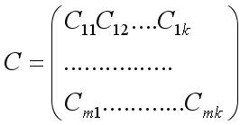

Where C 11 is the sum of pairwise products of the elements of a row of matrix A and a column of matrix B, that is, the element is the sum of the product of an element of the first column of the first row of matrix A with an element of the first column of the first row of matrix B, an element of the second column of the first row of matrix A with an element of the first column of the second row matrices B, etc.
When multiplying, the order of multiplication is important. A*B is not equal to B*A.

Finding the determinant.

Any square matrix can generate a determinant or a determinant. Writes det. Or | matrix elements |
For matrices of dimension 2 by 2. Determine there is a difference between the product of the elements of the main and the elements of the secondary diagonal.

For matrices with dimensions of 3 by 3 or more. The operation of finding the determinant is more complicated.
Let's introduce the concepts:
Element minor– is the determinant of a matrix obtained from the original matrix by crossing out the row and column of the original matrix in which this element was located.
Algebraic complement element of a matrix is ​​the product of the minor of this element by -1 to the power of the sum of the row and column of the original matrix in which this element was located.
The determinant of any square matrix is ​​equal to the sum of the product of the elements of any row of the matrix by their corresponding algebraic complements.

Matrix inversion

Matrix inversion is the process of finding the inverse of a matrix, the definition of which we gave at the beginning. The inverse matrix is ​​denoted in the same way as the original one with the addition of degree -1.
Find the inverse matrix using the formula.
A -1 = A * T x (1/|A|)
Where A * T is the Transposed Matrix of Algebraic Complements.

We made examples of solving matrices in the form of a video tutorial

:

If you want to figure it out, be sure to watch it.

These are the basic operations for solving matrices. If you have additional questions about how to solve matrices, feel free to write in the comments.

If you still can’t figure it out, try contacting a specialist.