A matrix polynomial in a variable is an expression of the form
F(l) = Ao lm + A1 lm-1 + A2 lm-2 + … + Am, (1)
where Ao, …, Am - square matrices of the same order with elements from the main field K. The number m is called the degree of a polynomial if Ao?0. Two polynomials are said to be equal if the matrices in these polynomials are equal equal degrees variable l. Matrix l-polynomials are added and multiplied by normal rules. It is clear that each l-polynomial can be written in the form of a single matrix, the elements of which are ordinary polynomials from l and vice versa. For example,
1 2 + 5 6 l + 1 0 lI = lI +5l + 1 6+ 2
0 3 7 -2 0 1 7l lI-2l + 3 .
Therefore, matrix n-polynomials are only special kind records of l-matrices.
The polynomial F(n) is called regular if the matrix Ao is invertible.
Sum (difference) of two matrix polynomials of the same order can be represented as a polynomial whose degree does not exceed the largest of the degrees of these polynomials.
The product of two matrix polynomials is equal to a polynomial whose degree is less than or equal to the sum of the degrees of the factors. If at least one of the two factors is a regular polynomial, then in this case the degree of the product is always equal to the sum of the degrees of the factors.
Let two matrix polynomials A(n) and B(n) of the same order n be given, and B(n) is a regular polynomial:
A(l) = Aolm + A1lm-1 + … + Am (Ao?0),
В(л) = Volr + В1лр-1 + … + Вр(|Во|?0).
We will say that the matrix polynomials Q(l) and R(l) are, respectively, the right quotient and the right remainder when dividing A(l) by B(l), if
A(l) = Q(l)B(l) + R(l)(2)
and the degree R(l) is less than the degree B(l).
In exactly the same way, we will call the polynomials ^Q(l) and ^R(l), respectively, the left quotient and the left remainder when dividing A(l) by B(l), if
A(l) = B(l) ^Q(l) + ^R(l)(3)
and the degree ^R(l) is less than the degree B(l).
IN general case the polynomials Q(l) and R(l) do not coincide with ^Q(l) and ^R(l).
Let us show that both right and left division of matrix polynomials of the same order are always feasible and unique if the divisor is a regular polynomial.
Consider the right division of A(n) by B(n). If m A(l)=AoBo -1lm-pB(l) + A(1)(l).(4) The degree m(1) of the polynomial A(1)(l) is less than m: A(1)(l) = Ao(1) lm(1) + … (Ao(1)?0, m(1) If m(1)?p, then repeating this process, we get: A(1)(l) = Ao(1)Bo -1 lm(1)-p B(l) + A(2)(l), (6) A(2)(l) = A(2)lm(2) + … (m(2) Since the degrees of the polynomials A(l), A(1)(l), A(2)(l), ... decrease, at some stage we will arrive at the remainder R(l), the degree of which is less than p. Then from (4), (6) it will follow: A(l) = Q(l) B(l) + R(l), where Q(l) = АoВо-1 lm-р + Ао(1)Во-1 lm(1)-р + …(7) Let us now prove the uniqueness of the right division. Let at the same time A(l) = Q(l) B(l) + R(l)(8) A(l) = Q*(l) B(l) + R*(l), (9) where the degrees of the polynomials R(l) and R*(l) are less than the degree B(l), i.e. less than p. Subtracting term by term (8) from (9) we get: B(l) = R*(l) - R(l).(10) If Q(l) - Q*(l) ? 0, then since |Во|?0, the degree of the left side of equality (10) would be equal to the sum of the degrees В(л) and Q(л) - Q*(л) and therefore would be?р. This is impossible, since the degree of the polynomial on the right side of equality (10) is less than p. Thus, Q(l) - Q*(l)?0, and then from (10) R*(l) - R(l)?0, i.e. Q(l) = Q*(l), R(l) = R*(l). The existence and uniqueness of the left quotient and left remainder are established in exactly the same way. Theorem 1. (Generalized Bezout's theorem). When a matrix polynomial F(n) is divided right (left) by a binomial lE-A, the remainder of the division is equal to F(A) (respectively ^F(A)). Proof. Consider an arbitrary matrix polynomial of nth order F(l) = Fо lm + F1 lm-1 + … + Fm (Fо?0)(11) This polynomial can also be written like this: F(l) = lm Fo + lm-1 F1 + … + Fm (12) Both entries for scalar l give the same result. However, if instead of the scalar argument l we substitute a square matrix of the nth order A, then the results of the substitution in (11) and (12) will be different, since the powers of the matrix A may not be commutable with the matrix coefficients Fo, F1, ..., Fm. F(A) = Fo Am+ F1 Am-1 + … + Fm (13) ^F(A) = Am Fо + Am-1 F1 + … + Fm(14) and we will call F(A) the right value, and ^F(A) the left value of the polynomial F(l) when substituting the matrix A for l. Let us divide the polynomial F(l) by the binomial le-A. In this case, the right remainder R and the left remainder ^R will not depend on l. To determine the right remainder, consider the usual division scheme: F(l) = Fo lm + F1 lm-1 + … + Fm = Fo lm-1(lE-A) + (Fo A + F1) lm-1 + F2 lm-2 + …= = (lE-A) + (Fо А2 + F1А1+ F2) lm-2 + F3 lm-3 + … = … … = (le-A) + Fо Аm + F1Аm-1 + … + Fm We found that R = Fо Аm+ F1Аm-1 + … + Fm = F(А).(15) Quite similar From the proven theorem it follows that the polynomial F(n) is divisible from the right (left) without a remainder by the binomial lE-A if and only if F(A)=0 (respectively ^F(A)=0). Check that A()=Q()B() + R(). А()= - 3 -2 2 +1 3 3 + = 1 2 3 + 0 1 2 + 1 0 + 0 0 1 3 -2 0 0 1 1 0 . 2 2 +3 - 2 +1 2 -1 2 + 3 1 В()= - 2 -1 2 +2 = -1 1 -1 2 , 1 1 3 5 2 +4 2 2 +13 |B o | = 1, B o -1 = 1 2, A 0 B 0 -1 = 2 5, A 0 B 0 -1 B() = - 2 +1 3 2 +12, 3 + 2 3 + 2 3 +4 2 3 +13 -3 2 -13 A (1) ()= - 3 -2 2 +1 3 3 + - - 3 + 3 3 +12 = -2 2 -+1 -11 , 0 1 2 + -3 -13 + 0 0 A (1) ()= -2 0 -1 -11 1 0 , A 0 (1) B 0 -1 ()= -2 0 1 2 = -2 -2, 1 2 2 2 +3 - 2 +1 = 1 2 +5 A 0 (1) B 0 -1 B()= -2 -2 - 2 -1 2 +1 -2 2 -4 -6 , R()= A (1) () - A 0 (1) B 0 -1 B()= 3 2 -13 - 1 2 +5 = -3-1 -13 -5 2 2 -+1 -11 -2 4 -4 -6 -+5 -11+6 , 3 5 + 1 2 3+1 5+2 Q() = A 0 B 0 -1 + A 0 (1) B 0 -1 = 2 5 -2 -2 = 2-2 5-2 Each square matrix has two polynomials associated with it: characteristic and minimal. These polynomials play an important role in various questions in matrix theory. So, for example, the concept of a function of a matrix, which we will introduce in the next chapter, will be entirely based on the concept of a minimal polynomial of a matrix. This chapter discusses the properties of characteristic and minimal polynomials. This study is preceded by basic information about polynomials with matrix coefficients and operations on them. Consider a square polynomial matrix, i.e. a square matrix whose elements are polynomials with respect to (with coefficients from a given number field): The matrix can be represented as a polynomial with matrix coefficients, arranged in powers: . (3) A number is called a degree of a polynomial if . The number is called the order of the polynomial. We will call a polynomial (1) regular if . We will sometimes call a polynomial with matrix coefficients a matrix polynomial. In contrast to the matrix polynomial, we will call an ordinary polynomial with scalar coefficients a scalar polynomial. Let's consider the basic operations on matrix polynomials. Let two matrix polynomials of the same order and be given. Let us denote by the largest of the powers of these polynomials. These polynomials can be written as that is, the sum (difference) of two matrix polynomials of the same order can be represented as a polynomial whose degree does not exceed the largest of the degrees of these polynomials. Let two matrix polynomials of degrees and the same order be given: If we multiplied by (that is, changed the order of the factors), then we would, generally speaking, get a different polynomial. Multiplying matrix polynomials has another specific property. In contrast to the product of scalar polynomials, the product of matrix polynomials (4) can have a degree less than , that is, less than the sum of the degrees of the factors. Indeed, in (4) the product of matrices can equal zero for and . However, if at least one of the matrices is non-singular, then it follows: . Thus, the product of two matrix polynomials is equal to a polynomial whose degree is less than or equal to the sum of the degrees of the factors. If at least one of the two factors is a regular polynomial, then in this case the degree of the product is always equal to the sum of the degrees of the factors. A matrix polynomial of the th order can be written in two ways: Both scalar entries give the same result. However, if we wish to substitute a square matrix of the th order instead of a scalar argument, then the results of substitutions in (5) and (5") will, generally speaking, be different, since the powers of the matrix may not be commutable with the matrix coefficients. and we will call the right and left values of the matrix polynomial when substituting instead of the matrix . Consider again the two matrix polynomials and their work The transformations in identity (7") remain valid when replaced by a matrix of the th order, if only the matrix commutes with all matrix coefficients. Similarly, in identity (7"), you can replace a scalar with a matrix if the matrix commutes with all coefficients. In the first case, we obtain: any matrix of the th order always satisfies the identities Instructions. For an online solution, you need to specify a matrix expression. At the second stage, it will be necessary to clarify the dimension of the matrices. Valid operations: multiplication (*), addition (+), subtraction (-), inverse matrix A^(-1), exponentiation (A^2, B^3), matrix transposition (A^T). A matrix is a rectangular numeric table with m rows and n columns, so the matrix can be schematically represented as a rectangle. Let's define basic operations on matrices. Example 6. . Example 7. Given matrices Example 8. Given a matrix § 1. Addition and multiplication of matrix polynomials
![]() ,
, ![]()
![]() ,
, ![]() . (9)
. (9)
To perform a list of operations, use a semicolon (;) separator. For example, to perform three operations:
a) 3A+4B
b) AB-VA
c) (A-B) -1
you will need to write it like this: 3*A+4*B;A*B-B*A;(A-B)^(-1)
Zero matrix (null matrix) is a matrix whose elements are all equal to zero and are denoted by 0.
Identity matrix is called a square matrix of the form
Two matrices A and B are equal, if they are the same size and their corresponding elements are equal.
Singular matrix is a matrix whose determinant is equal to zero (Δ = 0). Matrix addition
Definition . The sum of two matrices of the same size is a matrix of the same dimensions, the elements of which are found according to the formula ![]() . Denoted by C = A+B.
. Denoted by C = A+B.
The operation of matrix addition extends to the case of any number of terms. Obviously A+0=A .
Let us emphasize once again that only matrices of the same size can be added; For matrices of different sizes, the addition operation is not defined.Subtraction of matrices
Definition . The difference B-A of matrices B and A of the same size is a matrix C such that A+ C = B. Matrix multiplication
Definition . The product of a matrix by a number α is a matrix obtained from A by multiplying all its elements by α, .
Definition . Let two matrices be given ![]()
![]() and , and the number of columns of A is equal to the number of rows of B. The product of A by B is a matrix whose elements are found according to the formula
and , and the number of columns of A is equal to the number of rows of B. The product of A by B is a matrix whose elements are found according to the formula  .
.
Denoted by C = A·B.
Schematically, the operation of matrix multiplication can be depicted as follows: 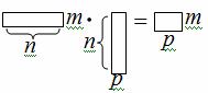
and the rule for calculating an element in a product: 
Let us emphasize once again that the product A·B makes sense if and only if the number of columns of the first factor is equal to the number of rows of the second, and the product produces a matrix whose number of rows is equal to the number of rows of the first factor, and the number of columns is equal to the number of columns of the second. You can check the result of multiplication using a special online calculator.  And
And  . Find matrices C = A·B and D = B·A.
Solution.
First of all, note that the product A·B exists because the number of columns of A is equal to the number of rows of B.
Note that in the general case A·B≠B·A, i.e. the product of matrices is anticommutative.
Let's find B·A (multiplication is possible).  . Find 3A 2 – 2A.
Solution.
 .
.
 ;
;  .
.
 .
.
Let us note the following interesting fact.
As you know, the product of two non-zero numbers is not equal to zero. For matrices, a similar circumstance may not occur, that is, the product of non-zero matrices may turn out to be equal to the null matrix.


