Systems of equations are widely used in the economic sector for mathematical modeling of various processes. For example, when solving problems of production management and planning, logistics routes (transport problem) or equipment placement.
Systems of equations are used not only in mathematics, but also in physics, chemistry and biology, when solving problems of finding population size.
A system of linear equations is two or more equations with several variables for which it is necessary to find a common solution. Such a sequence of numbers for which all equations become true equalities or prove that the sequence does not exist.
Linear equation
Equations of the form ax+by=c are called linear. The designations x, y are the unknowns whose value must be found, b, a are the coefficients of the variables, c is the free term of the equation.
Solving an equation by plotting it will look like a straight line, all points of which are solutions to the polynomial.
Types of systems of linear equations
The simplest examples are considered to be systems of linear equations with two variables X and Y.
F1(x, y) = 0 and F2(x, y) = 0, where F1,2 are functions and (x, y) are function variables.
Solve system of equations - this means finding values (x, y) at which the system turns into a true equality or establishing that suitable values of x and y do not exist.
A pair of values (x, y), written as the coordinates of a point, is called a solution to a system of linear equations.
If systems have one common solution or no solution exists, they are called equivalent.
Homogeneous systems of linear equations are systems whose right-hand side is equal to zero. If the right part after the equal sign has a value or is expressed by a function, such a system is heterogeneous.
The number of variables can be much more than two, then we should talk about an example of a system of linear equations with three or more variables.
When faced with systems, schoolchildren assume that the number of equations must necessarily coincide with the number of unknowns, but this is not the case. The number of equations in the system does not depend on the variables; there can be as many of them as desired.
Simple and complex methods for solving systems of equations
There is no general analytical method for solving such systems; all methods are based on numerical solutions. The school mathematics course describes in detail such methods as permutation, algebraic addition, substitution, as well as graphical and matrix methods, solution by the Gaussian method.
The main task when teaching solution methods is to teach how to correctly analyze the system and find the optimal solution algorithm for each example. The main thing is not to memorize a system of rules and actions for each method, but to understand the principles of using a particular method
Solving examples of systems of linear equations in the 7th grade general education curriculum is quite simple and explained in great detail. In any mathematics textbook, this section is given enough attention. Solving examples of systems of linear equations using the Gauss and Cramer method is studied in more detail in the first years of higher education.
Solving systems using the substitution method
The actions of the substitution method are aimed at expressing the value of one variable in terms of the second. The expression is substituted into the remaining equation, then it is reduced to a form with one variable. The action is repeated depending on the number of unknowns in the system
Let us give a solution to an example of a system of linear equations of class 7 using the substitution method:

As can be seen from the example, the variable x was expressed through F(X) = 7 + Y. The resulting expression, substituted into the 2nd equation of the system in place of X, helped to obtain one variable Y in the 2nd equation. Solving this example is easy and allows you to get the Y value. The last step is to check the obtained values.
It is not always possible to solve an example of a system of linear equations by substitution. The equations can be complex and expressing the variable in terms of the second unknown will be too cumbersome for further calculations. When there are more than 3 unknowns in the system, solving by substitution is also inappropriate.
Solution of an example of a system of linear inhomogeneous equations:

Solution using algebraic addition
When searching for solutions to systems using the addition method, equations are added term by term and multiplied by various numbers. The ultimate goal of mathematical operations is an equation in one variable.

Application of this method requires practice and observation. Solving a system of linear equations using the addition method when there are 3 or more variables is not easy. Algebraic addition is convenient to use when equations contain fractions and decimals.
Solution algorithm:
- Multiply both sides of the equation by a certain number. As a result of the arithmetic operation, one of the coefficients of the variable should become equal to 1.
- Add the resulting expression term by term and find one of the unknowns.
- Substitute the resulting value into the 2nd equation of the system to find the remaining variable.
Method of solution by introducing a new variable
A new variable can be introduced if the system requires finding a solution for no more than two equations; the number of unknowns should also be no more than two.
The method is used to simplify one of the equations by introducing a new variable. The new equation is solved for the introduced unknown, and the resulting value is used to determine the original variable.

The example shows that by introducing a new variable t, it was possible to reduce the 1st equation of the system to a standard quadratic trinomial. You can solve a polynomial by finding the discriminant.
It is necessary to find the value of the discriminant using the well-known formula: D = b2 - 4*a*c, where D is the desired discriminant, b, a, c are the factors of the polynomial. In the given example, a=1, b=16, c=39, therefore D=100. If the discriminant is greater than zero, then there are two solutions: t = -b±√D / 2*a, if the discriminant is less than zero, then there is one solution: x = -b / 2*a.
The solution for the resulting systems is found by the addition method.
Visual method for solving systems
Suitable for 3 equation systems. The method consists in constructing graphs of each equation included in the system on the coordinate axis. The coordinates of the intersection points of the curves will be the general solution of the system.
The graphical method has a number of nuances. Let's look at several examples of solving systems of linear equations in a visual way.

As can be seen from the example, for each line two points were constructed, the values of the variable x were chosen arbitrarily: 0 and 3. Based on the values of x, the values for y were found: 3 and 0. Points with coordinates (0, 3) and (3, 0) were marked on the graph and connected by a line.
The steps must be repeated for the second equation. The point of intersection of the lines is the solution of the system.
The following example requires finding a graphical solution to a system of linear equations: 0.5x-y+2=0 and 0.5x-y-1=0.

As can be seen from the example, the system has no solution, because the graphs are parallel and do not intersect along their entire length.

The systems from examples 2 and 3 are similar, but when constructed it becomes obvious that their solutions are different. It should be remembered that it is not always possible to say whether a system has a solution or not; it is always necessary to construct a graph.
The matrix and its varieties
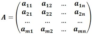
Matrices are used to concisely write a system of linear equations. A matrix is a special type of table filled with numbers. n*m has n - rows and m - columns.
A matrix is square when the number of columns and rows are equal. A matrix-vector is a matrix of one column with an infinitely possible number of rows. A matrix with ones along one of the diagonals and other zero elements is called identity.
An inverse matrix is a matrix, when multiplied by which the original one turns into a unit matrix; such a matrix exists only for the original square one.
Rules for converting a system of equations into a matrix
In relation to systems of equations, the coefficients and free terms of the equations are written as matrix numbers; one equation is one row of the matrix.
A matrix row is said to be nonzero if at least one element of the row is not zero. Therefore, if in any of the equations the number of variables differs, then it is necessary to enter zero in place of the missing unknown.
The matrix columns must strictly correspond to the variables. This means that the coefficients of the variable x can be written only in one column, for example the first, the coefficient of the unknown y - only in the second.
When multiplying a matrix, all elements of the matrix are sequentially multiplied by a number.
Options for finding the inverse matrix
The formula for finding the inverse matrix is quite simple: K -1 = 1 / |K|, where K -1 is the inverse matrix, and |K| is the determinant of the matrix. |K| must not be equal to zero, then the system has a solution.
The determinant is easily calculated for a two-by-two matrix; you just need to multiply the diagonal elements by each other. For the “three by three” option there is a formula |K|=a 1 b 2 c 3 + a 1 b 3 c 2 + a 3 b 1 c 2 + a 2 b 3 c 1 + a 2 b 1 c 3 + a 3 b 2 c 1 . You can use the formula, or you can remember that you need to take one element from each row and each column so that the numbers of columns and rows of elements are not repeated in the work.
Solving examples of systems of linear equations using the matrix method
The matrix method of finding a solution allows you to reduce cumbersome entries when solving systems with a large number of variables and equations.

In the example, a nm are the coefficients of the equations, the matrix is a vector x n are variables, and b n are free terms.


Solving systems using the Gaussian method
In higher mathematics, the Gaussian method is studied together with the Cramer method, and the process of finding solutions to systems is called the Gauss-Cramer solution method. These methods are used to find variables of systems with a large number of linear equations.
The Gauss method is very similar to solutions by substitution and algebraic addition, but is more systematic. In the school course, the solution by the Gaussian method is used for systems of 3 and 4 equations. The purpose of the method is to reduce the system to the form of an inverted trapezoid. By means of algebraic transformations and substitutions, the value of one variable is found in one of the equations of the system. The second equation is an expression with 2 unknowns, while 3 and 4 are, respectively, with 3 and 4 variables.
After bringing the system to the described form, the further solution is reduced to the sequential substitution of known variables into the equations of the system.
In school textbooks for grade 7, an example of a solution by the Gauss method is described as follows:

As can be seen from the example, at step (3) two equations were obtained: 3x 3 -2x 4 =11 and 3x 3 +2x 4 =7. Solving any of the equations will allow you to find out one of the variables x n.

Theorem 5, which is mentioned in the text, states that if one of the equations of the system is replaced by an equivalent one, then the resulting system will also be equivalent to the original one.
The Gaussian method is difficult for middle school students to understand, but it is one of the most interesting ways to develop the ingenuity of children enrolled in advanced learning programs in math and physics classes.
For ease of recording, calculations are usually done as follows:

The coefficients of the equations and free terms are written in the form of a matrix, where each row of the matrix corresponds to one of the equations of the system. separates the left side of the equation from the right. Roman numerals indicate the numbers of equations in the system.
First, write down the matrix to be worked with, then all the actions carried out with one of the rows. The resulting matrix is written after the "arrow" sign and the necessary algebraic operations are continued until the result is achieved.
The result should be a matrix in which one of the diagonals is equal to 1, and all other coefficients are equal to zero, that is, the matrix is reduced to a unit form. We must not forget to perform calculations with numbers on both sides of the equation.
This recording method is less cumbersome and allows you not to be distracted by listing numerous unknowns.
The free use of any solution method will require care and some experience. Not all methods are of an applied nature. Some methods of finding solutions are more preferable in a particular area of human activity, while others exist for educational purposes.
If a problem has fewer than three variables, it is not a problem; if it is more than eight, it is unsolvable. Enon.
Problems with parameters are found in all versions of the Unified State Exam, since solving them most clearly reveals how deep and informal the graduate’s knowledge is. The difficulties that students encounter when completing such tasks are caused not only by their relative complexity, but also by the fact that insufficient attention is paid to them in textbooks. In the versions of KIMs in mathematics, there are two types of tasks with parameters. The first: “for each value of the parameter, solve the equation, inequality or system.” The second: “find all values of the parameter, for each of which the solutions to the inequality, equation or system satisfy the given conditions.” Accordingly, the answers in problems of these two types differ in essence. In the first case, the answer lists all possible values of the parameter and for each of these values the solutions to the equation are written. The second lists all parameter values at which the conditions of the problem are met. Writing down the answer is an essential stage of the solution; it is very important not to forget to reflect all stages of the solution in the answer. Students need to pay attention to this.
The appendix to the lesson contains additional material on the topic “Solving systems of linear equations with parameters”, which will help in preparing students for the final certification.
Lesson objectives:
- systematization of students' knowledge;
- developing the ability to use graphical representations when solving systems of equations;
- developing the ability to solve systems of linear equations containing parameters;
- implementation of operational control and self-control of students;
- development of research and cognitive activity of schoolchildren, the ability to evaluate the results obtained.
The lesson lasts two hours.
Lesson progress
- Organizational moment
Communicate the topic, goals and objectives of the lesson.
- Updating students' basic knowledge
Checking homework. As homework, students were asked to solve each of three systems of linear equations
a) b) ![]() V)
V) ![]()
graphically and analytically; draw a conclusion about the number of solutions obtained for each case
The conclusions made by students are listened to and analyzed. The results of the work under the guidance of the teacher are summarized in notebooks.
In general, a system of two linear equations with two unknowns can be represented as: ![]() .
.
Solving a given system of equations graphically means finding the coordinates of the intersection points of the graphs of these equations or proving that there are none. The graph of each equation of this system on a plane is a certain straight line.
There are three possible cases of mutual arrangement of two straight lines on a plane:

<Рисунок1>;

<Рисунок2>;
<Рисунок3>.
For each case it is useful to make a drawing.
- Learning new material
Today in the lesson we will learn how to solve systems of linear equations containing parameters. We will call a parameter an independent variable, the value of which in the problem is considered to be a given fixed or arbitrary real number, or a number belonging to a predetermined set. Solving a system of equations with a parameter means establishing a correspondence that allows for any value of the parameter to find the corresponding set of solutions to the system.
The solution to a problem with a parameter depends on the question posed in it. If you simply need to solve a system of equations for different values of a parameter or study it, then you need to give a substantiated answer for any value of the parameter or for the value of a parameter belonging to a set previously specified in the problem. If it is necessary to find parameter values that satisfy certain conditions, then a complete study is not required, and the solution of the system is limited to finding these specific parameter values.
Example 1. For each parameter value, we solve the system of equations
![]()
Solution.
- The system has a unique solution if
In this case we have
![]()
- If a = 0, then the system takes the form
![]()
The system is inconsistent, i.e. has no solutions.
- If then the system is written in the form
Obviously, in this case the system has infinitely many solutions of the form x = t; where t is any real number.
Answer:
Example 2.
- has a unique solution;
- has many solutions;
- has no solutions?
Solution.
Answer:
Example 3. Let us find the sum of parameters a and b for which the system
![]()
has countless solutions.
Solution. The system has infinitely many solutions if
That is, if a = 12, b = 36; a + b = 12 + 36 =48.
Answer: 48.
- Consolidating what has been learned while solving problems
- No. 15.24(a) . For each parameter value, solve the system of equations
![]()
- No. 15.25(a) For each parameter value, solve the system of equations
![]()
- At what values of parameter a does the system of equations
![]()
a) has no solutions; b) has infinitely many solutions.
Answer: for a = 2 there are no solutions, for a = -2 there is an infinite number of solutions
- Practical work in groups
The class is divided into groups of 4-5 people. Each group includes students with different levels of mathematical preparation. Each group receives a task card. You can invite all groups to solve one system of equations, and formalize the solution. The group that was the first to correctly complete the task presents its solution; the rest hand over the solution to the teacher.
Card. Solve system of linear equations
![]()
for all values of parameter a.
Answer: when ![]() the system has a unique solution
the system has a unique solution ![]() ; when there are no solutions; for a = -1 there are infinitely many solutions of the form, (t; 1- t) where t R
; when there are no solutions; for a = -1 there are infinitely many solutions of the form, (t; 1- t) where t R
If the class is strong, the groups may be offered different systems of equations, the list of which is in Appendix1. Then each group presents their solution to the class.
Report of the group that was the first to correctly complete the task
Participants voice and explain their solution and answer questions raised by representatives of other groups.
- Independent work
Option 1
Option 2
- Lesson summary
Solving systems of linear equations with parameters can be compared to a study that involves three basic conditions. The teacher invites students to formulate them.
When deciding, remember:
- In order for a system to have a unique solution, it is necessary that the lines corresponding to the equation of the system intersect, i.e. the condition must be met;
- in order to have no solutions, the lines must be parallel, i.e. the condition was met
- and, finally, for a system to have infinitely many solutions, the lines must coincide, i.e. the condition was met.
The teacher evaluates the work of the class as a whole and assigns marks for the lesson to individual students. After checking their independent work, each student will receive a grade for the lesson.
- Homework
At what values of the parameter b does the system of equations ![]()
- has infinitely many solutions;
- has no solutions?
The graphs of the functions y = 4x + b and y = kx + 6 are symmetrical about the ordinate.
- Find b and k,
- find the coordinates of the intersection point of these graphs.
Solve the system of equations for all values of m and n.
Solve a system of linear equations for all values of the parameter a (any value of your choice).
Literature
- Algebra and the beginnings of mathematical analysis: textbook. for 11th grade general education institutions: basic and profile. levels / S. M. Nikolsky, M. K. Potapov, N. N. Reshetnikov, A. V. Shevkin - M.: Education, 2008.
- Mathematics: 9th grade: Preparation for the state final certification / M. N. Korchagina, V. V. Korchagin - M.: Eksmo, 2008.
- We are preparing for university. Mathematics. Part 2. A textbook for preparing for the Unified State Exam, participation in centralized testing and passing entrance tests to Kuban State Technical University / Kuban. state technol. University; Institute of modern technol. and econ.; Compiled by: S. N. Gorshkova, L. M. Danovich, N. A. Naumova, A.V. Martynenko, I.A. Palshchikova. – Krasnodar, 2006.
- Collection of problems in mathematics for TUSUR preparatory courses: Textbook / Z. M. Goldshtein, G. A. Kornievskaya, G. A. Korotchenko, S. N. Kudinova. – Tomsk: Tomsk. State University of Control Systems and Radioelectronics, 1998.
- Mathematics: intensive exam preparation course / O. Yu. Cherkasov, A. G. Yakushev. – M.: Rolf, Iris-press, 1998.
Solution. A=  . Let's find r(A). Because matrix And has order 3x4, then the highest order of minors is 3. Moreover, all third-order minors are equal to zero (check it yourself). Means, r(A)< 3. Возьмем главный basic minor = -5-4 = -9 ≠
0. Therefore r(A) =2.
. Let's find r(A). Because matrix And has order 3x4, then the highest order of minors is 3. Moreover, all third-order minors are equal to zero (check it yourself). Means, r(A)< 3. Возьмем главный basic minor = -5-4 = -9 ≠
0. Therefore r(A) =2.
Let's consider matrix WITH =  .
.
Minor third order ≠ 0. So r(C) = 3.
Since r(A) ≠ r(C) , then the system is inconsistent.
Example 2. Determine the compatibility of a system of equations 
Solve this system if it turns out to be consistent.
Solution.
A = , C =  . It is obvious that r(A) ≤ 3, r(C) ≤ 4. Since detC = 0, then r(C)< 4. Let's consider minor third order, located in the upper left corner of the matrix A and C: = -23 ≠
0. So r(A) = r(C) = 3.
. It is obvious that r(A) ≤ 3, r(C) ≤ 4. Since detC = 0, then r(C)< 4. Let's consider minor third order, located in the upper left corner of the matrix A and C: = -23 ≠
0. So r(A) = r(C) = 3.
Number unknown in system n=3. This means that the system has a unique solution. In this case, the fourth equation represents the sum of the first three and can be ignored.
According to Cramer's formulas we get x 1 = -98/23, x 2 = -47/23, x 3 = -123/23.
2.4. Matrix method. Gaussian method
system n linear equations With n unknowns can be solved matrix method according to the formula X = A -1 B (at Δ ≠ 0), which is obtained from (2) by multiplying both parts by A -1.
Example 1. Solve a system of equations 
matrix method (in section 2.2 this system was solved using Cramer’s formulas)
Solution. Δ = 10 ≠ 0 A = - non-degenerate matrix.
=  (check this yourself by making the necessary calculations).
A -1 = (1/Δ)х=  .
.
X = A -1 V = x= .
Answer: .
From a practical point of view matrix method and formulas Kramer are associated with a large amount of computation, so preference is given Gaussian method, which consists in the sequential elimination of unknowns. To do this, the system of equations is reduced to an equivalent system with a triangular extended matrix (all elements below the main diagonal are equal to zero). These actions are called forward movement. From the resulting triangular system, the variables are found using successive substitutions (reverse).
Example 2. Solve the system using the Gauss method
(Above, this system was solved using Cramer’s formula and the matrix method).
Solution.
Direct move. Let us write down the extended matrix and, using elementary transformations, reduce it to triangular form:
 ~
~  ~
~  ~
~  ~
~  .
.
We get system 
Reverse move. From the last equation we find X 3 = -6 and substitute this value into the second equation:
X 2 = - 11/2 - 1/4X 3 = - 11/2 - 1/4(-6) = - 11/2 + 3/2 = -8/2 = -4.
X 1 = 2 -X 2 + X 3 = 2+4-6 = 0.
Answer: .
2.5. General solution of a system of linear equations
Let a system of linear equations be given = b i(i=). Let r(A) = r(C) = r, i.e. the system is collaborative. Any minor of order r other than zero is basic minor. Without loss of generality, we will assume that the basis minor is located in the first r (1 ≤ r ≤ min(m,n)) rows and columns of matrix A. Having discarded the last m-r equations of the system, we write a shortened system:

which is equivalent to the original one. Let's name the unknowns x 1 ,….x r basic, and x r +1 ,…, x r free and move the terms containing free unknowns to the right side of the equations of the truncated system. We obtain a system with respect to the basic unknowns:

which for each set of values of free unknowns x r +1 = С 1 ,…, x n = С n-r has only one solution x 1 (C 1 ,…, C n-r),…, x r (C 1 ,…, C n-r), found by Cramer's rule.
Corresponding Solution the shortened, and therefore the original system has the form:
X(C 1 ,…, C n-r) =  -
general solution of the system.
-
general solution of the system.
If in the general solution we assign some numerical values to the free unknowns, we obtain a solution to the linear system, called a partial solution.
Example. Establish compatibility and find a general solution of the system

Solution. A =  , C =
, C =  .
.
So How r(A)= r(C) = 2 (see this for yourself), then the original system is consistent and has an infinite number of solutions (since r< 4).
Example 1. Find a general solution and some particular solution of the systemSolution We do it using a calculator. Let's write out the extended and main matrices: 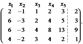
The main matrix A is separated by a dotted line. We write unknown systems at the top, keeping in mind the possible rearrangement of terms in the equations of the system. By determining the rank of the extended matrix, we simultaneously find the rank of the main one. In matrix B, the first and second columns are proportional. Of the two proportional columns, only one can fall into the basic minor, so let’s move, for example, the first column beyond the dotted line with the opposite sign. For the system, this means transferring terms from x 1 to the right side of the equations. 
Let's reduce the matrix to triangular form. We will work only with rows, since multiplying a matrix row by a number other than zero and adding it to another row for the system means multiplying the equation by the same number and adding it with another equation, which does not change the solution of the system. We work with the first row: multiply the first row of the matrix by (-3) and add to the second and third rows in turn. Then multiply the first line by (-2) and add it to the fourth. 
The second and third lines are proportional, therefore, one of them, for example the second, can be crossed out. This is equivalent to crossing out the second equation of the system, since it is a consequence of the third. 
Now we work with the second line: multiply it by (-1) and add it to the third. 
The minor circled with a dotted line has the highest order (of possible minors) and is non-zero (it is equal to the product of the elements on the main diagonal), and this minor belongs to both the main matrix and the extended one, therefore rangA = rangB = 3.
Minor  is basic. It includes coefficients for the unknowns x 2 , x 3 , x 4 , which means that the unknowns x 2 , x 3 , x 4 are dependent, and x 1 , x 5 are free.
Let's transform the matrix, leaving only the basis minor on the left (which corresponds to point 4 of the above solution algorithm). 
The system with the coefficients of this matrix is equivalent to the original system and has the form
Using the method of eliminating unknowns we find: ![]() , ,
, ,
We obtained relations expressing the dependent variables x 2, x 3, x 4 through the free ones x 1 and x 5, that is, we found a general solution: 
By assigning any values to the free unknowns, we obtain any number of particular solutions. Let's find two particular solutions:
1) let x 1 = x 5 = 0, then x 2 = 1, x 3 = -3, x 4 = 3;
2) put x 1 = 1, x 5 = -1, then x 2 = 4, x 3 = -7, x 4 = 7.
Thus, two solutions were found: (0,1,-3,3,0) – one solution, (1,4,-7,7,-1) – another solution.
Example 2. Explore compatibility, find a general and one particular solution to the system 
Solution. Let's rearrange the first and second equations to have one in the first equation and write the matrix B. 
We get zeros in the fourth column by operating with the first row: 
Now we get the zeros in the third column using the second line: 
 The third and fourth lines are proportional, so one of them can be crossed out without changing the rank:
Multiply the third line by (–2) and add it to the fourth: 
We see that the ranks of the main and extended matrices are equal to 4, and the rank coincides with the number of unknowns, therefore, the system has a unique solution:
;
x 4 = 10- 3x 1 – 3x 2 – 2x 3 = 11.
Example 3. Examine the system for compatibility and find a solution if it exists. 
Solution. We compose an extended matrix of the system. 
 We rearrange the first two equations so that there is 1 in the upper left corner:
Multiplying the first line by (-1), adding it to the third: 
Multiply the second line by (-2) and add it to the third: 
The system is inconsistent, since in the main matrix we received a row consisting of zeros, which is crossed out when the rank is found, but in the extended matrix the last row remains, that is, r B > r A .
Exercise. Investigate this system of equations for compatibility and solve it using matrix calculus.
Solution
Example. Prove the compatibility of the system of linear equations and solve it in two ways: 1) by the Gauss method; 2) Cramer's method. (enter the answer in the form: x1,x2,x3)
Solution :doc :doc :xls
Answer: 2,-1,3.
Example. A system of linear equations is given. Prove its compatibility. Find a general solution of the system and one particular solution.
Solution
Answer: x 3 = - 1 + x 4 + x 5 ; x 2 = 1 - x 4 ; x 1 = 2 + x 4 - 3x 5
Exercise. Find the general and particular solutions of each system.
Solution. We study this system using the Kronecker-Capelli theorem.
Let's write out the extended and main matrices:
| 1 | 1 | 14 | 0 | 2 | 0 |
| 3 | 4 | 2 | 3 | 0 | 1 |
| 2 | 3 | -3 | 3 | -2 | 1 |
| x 1 | x 2 | x 3 | x 4 | x 5 |
Here matrix A is highlighted in bold.
Let's reduce the matrix to triangular form. We will work only with rows, since multiplying a matrix row by a number other than zero and adding it to another row for the system means multiplying the equation by the same number and adding it with another equation, which does not change the solution of the system.
Let's multiply the 1st line by (3). Multiply the 2nd line by (-1). Let's add the 2nd line to the 1st:
| 0 | -1 | 40 | -3 | 6 | -1 |
| 3 | 4 | 2 | 3 | 0 | 1 |
| 2 | 3 | -3 | 3 | -2 | 1 |
Let's multiply the 2nd line by (2). Multiply the 3rd line by (-3). Let's add the 3rd line to the 2nd:
| 0 | -1 | 40 | -3 | 6 | -1 |
| 0 | -1 | 13 | -3 | 6 | -1 |
| 2 | 3 | -3 | 3 | -2 | 1 |
Multiply the 2nd line by (-1). Let's add the 2nd line to the 1st:
| 0 | 0 | 27 | 0 | 0 | 0 |
| 0 | -1 | 13 | -3 | 6 | -1 |
| 2 | 3 | -3 | 3 | -2 | 1 |
The selected minor has the highest order (of possible minors) and is non-zero (it is equal to the product of the elements on the reverse diagonal), and this minor belongs to both the main matrix and the extended one, therefore rang(A) = rang(B) = 3 Since the rank of the main matrix is equal to the rank of the extended one, then the system is collaborative.
This minor is basic. It includes coefficients for the unknowns x 1 , x 2 , x 3 , which means that the unknowns x 1 , x 2 , x 3 are dependent (basic), and x 4 , x 5 are free.
Let's transform the matrix, leaving only the basis minor on the left.
| 0 | 0 | 27 | 0 | 0 | 0 |
| 0 | -1 | 13 | -1 | 3 | -6 |
| 2 | 3 | -3 | 1 | -3 | 2 |
| x 1 | x 2 | x 3 | x 4 | x 5 |
27x 3 =
- x 2 + 13x 3 = - 1 + 3x 4 - 6x 5
2x 1 + 3x 2 - 3x 3 = 1 - 3x 4 + 2x 5
Using the method of eliminating unknowns we find:
We obtained relations expressing the dependent variables x 1 , x 2 , x 3 through the free ones x 4 , x 5 , that is, we found general solution:
x 3 = 0
x 2 = 1 - 3x 4 + 6x 5
x 1 = - 1 + 3x 4 - 8x 5
uncertain, because has more than one solution.
Exercise. Solve the system of equations.
Answer:x 2 = 2 - 1.67x 3 + 0.67x 4
x 1 = 5 - 3.67x 3 + 0.67x 4
By assigning any values to the free unknowns, we obtain any number of particular solutions. The system is uncertain
- Systems m linear equations with n unknown.
Solving a system of linear equations- this is such a set of numbers ( x 1 , x 2 , …, x n), when substituted into each of the equations of the system, the correct equality is obtained.
Where a ij , i = 1, …, m; j = 1, …, n— system coefficients;
b i , i = 1, …, m- free members;
x j , j = 1, …, n- unknown.
The above system can be written in matrix form: A X = B,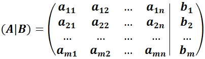
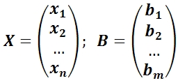
Where ( A|B) is the main matrix of the system;
A— extended system matrix;
X— column of unknowns;
B— column of free members.
If matrix B is not a null matrix ∅, then this system of linear equations is called inhomogeneous.
If matrix B= ∅, then this system of linear equations is called homogeneous. A homogeneous system always has a zero (trivial) solution: x 1 = x 2 = …, x n = 0.
Joint system of linear equations is a system of linear equations that has a solution.
Inconsistent system of linear equations is an unsolvable system of linear equations.
A certain system of linear equations is a system of linear equations that has a unique solution.
Indefinite system of linear equations is a system of linear equations with an infinite number of solutions. - Systems of n linear equations with n unknowns
If the number of unknowns is equal to the number of equations, then the matrix is square. The determinant of a matrix is called the main determinant of a system of linear equations and is denoted by the symbol Δ.
Cramer method for solving systems n linear equations with n unknown.
Cramer's rule.
If the main determinant of a system of linear equations is not equal to zero, then the system is consistent and defined, and the only solution is calculated using the Cramer formulas:
where Δ i are determinants obtained from the main determinant of the system Δ by replacing i th column to the column of free members. . - Systems of m linear equations with n unknowns
Kronecker–Capelli theorem.
In order for a given system of linear equations to be consistent, it is necessary and sufficient that the rank of the system matrix be equal to the rank of the extended matrix of the system, rang(Α) = rang(Α|B).
If rang(Α) ≠ rang(Α|B), then the system obviously has no solutions.
If rang(Α) = rang(Α|B), then two cases are possible:
1) rank(Α) = n(number of unknowns) - the solution is unique and can be obtained using Cramer’s formulas;
2) rank(Α)< n - there are infinitely many solutions. - Gauss method for solving systems of linear equations
Let's create an extended matrix ( A|B) of a given system from the coefficients of the unknowns and the right-hand sides.
The Gaussian method or the method of eliminating unknowns consists of reducing the extended matrix ( A|B) using elementary transformations over its rows to a diagonal form (to the upper triangular form). Returning to the system of equations, all unknowns are determined.
Elementary transformations over strings include the following:
1) swapping two lines;
2) multiplying a string by a number other than 0;
3) adding another string to a string, multiplied by an arbitrary number;
4) throwing out a zero line.
An extended matrix reduced to diagonal form corresponds to a linear system equivalent to the given one, the solution of which does not cause difficulties. . - System of homogeneous linear equations.
A homogeneous system has the form:
it corresponds to the matrix equation A X = 0.
1) A homogeneous system is always consistent, since r(A) = r(A|B), there is always a zero solution (0, 0, …, 0).
2) In order for a homogeneous system to have a non-zero solution, it is necessary and sufficient that r = r(A)< n , which is equivalent to Δ = 0.
3) If r< n , then obviously Δ = 0, then free unknowns arise c 1, c 2, …, c n-r, the system has non-trivial solutions, and there are infinitely many of them.
4) General solution X at r< n can be written in matrix form as follows:
X = c 1 X 1 + c 2 X 2 + … + c n-r X n-r,
where are the solutions X 1 , X 2 , …, X n-r form a fundamental system of solutions.
5) The fundamental system of solutions can be obtained from the general solution of a homogeneous system: ,
,
if we sequentially set the parameter values equal to (1, 0, …, 0), (0, 1, …, 0), …, (0, 0, …, 1).
Expansion of the general solution in terms of the fundamental system of solutions is a record of a general solution in the form of a linear combination of solutions belonging to the fundamental system.
Theorem. In order for a system of linear homogeneous equations to have a non-zero solution, it is necessary and sufficient that Δ ≠ 0.
So, if the determinant Δ ≠ 0, then the system has a unique solution.
If Δ ≠ 0, then the system of linear homogeneous equations has an infinite number of solutions.
Theorem. In order for a homogeneous system to have a nonzero solution, it is necessary and sufficient that r(A)< n .
Proof:
1) r there can't be more n(the rank of the matrix does not exceed the number of columns or rows);
2) r< n , because If r = n, then the main determinant of the system Δ ≠ 0, and, according to Cramer’s formulas, there is a unique trivial solution x 1 = x 2 = … = x n = 0, which contradicts the condition. Means, r(A)< n .
Consequence. In order for a homogeneous system n linear equations with n unknowns had a non-zero solution, it is necessary and sufficient that Δ = 0.


