I. Ordinary differential equations
1.1. Basic concepts and definitions
A differential equation is an equation that relates an independent variable x, the required function y and its derivatives or differentials.
Symbolically, the differential equation is written as follows:
F(x,y,y")=0, F(x,y,y")=0, F(x,y,y",y",.., y (n))=0
A differential equation is called ordinary if the required function depends on one independent variable.
Solving a differential equation is called a function that turns this equation into an identity.
The order of the differential equation is the order of the highest derivative included in this equation
Examples.
1. Consider a first order differential equation
The solution to this equation is the function y = 5 ln x. Indeed, substituting y" into the equation, we get the identity.
And this means that the function y = 5 ln x– is a solution to this differential equation.
2. Consider the second order differential equation y" - 5y" +6y = 0. The function is the solution to this equation.
Really, .
Substituting these expressions into the equation, we obtain: , – identity.
And this means that the function is the solution to this differential equation.
Integrating differential equations is the process of finding solutions to differential equations.
General solution of the differential equation called a function of the form ![]() , which includes as many independent arbitrary constants as the order of the equation.
, which includes as many independent arbitrary constants as the order of the equation.
Partial solution of the differential equation is a solution obtained from a general solution for various numerical values of arbitrary constants. The values of arbitrary constants are found at certain initial values of the argument and function.
The graph of a particular solution to a differential equation is called integral curve.
Examples
1. Find a particular solution to a first order differential equation
xdx + ydy = 0, If y= 4 at x = 3.
Solution. Integrating both sides of the equation, we get
Comment. An arbitrary constant C obtained as a result of integration can be represented in any form convenient for further transformations. In this case, taking into account the canonical equation of a circle, it is convenient to represent an arbitrary constant C in the form .
![]() - general solution of the differential equation.
- general solution of the differential equation.
Particular solution of the equation satisfying the initial conditions y = 4 at x = 3 is found from the general by substituting the initial conditions into the general solution: 3 2 + 4 2 = C 2 ; C=5.
Substituting C=5 into the general solution, we get x 2 +y 2 = 5 2 .
This is a particular solution to a differential equation obtained from a general solution under given initial conditions.
2. Find the general solution to the differential equation
The solution to this equation is any function of the form , where C is an arbitrary constant. Indeed, substituting , into the equations, we obtain: , .
Consequently, this differential equation has an infinite number of solutions, since for different values of the constant C, equality determines different solutions to the equation.
For example, by direct substitution you can verify that the functions ![]() are solutions to the equation.
are solutions to the equation.
A problem in which you need to find a particular solution to the equation y" = f(x,y) satisfying the initial condition y(x 0) = y 0, is called the Cauchy problem.
Solving the equation y" = f(x,y), satisfying the initial condition, y(x 0) = y 0, is called a solution to the Cauchy problem.
The solution to the Cauchy problem has a simple geometric meaning. Indeed, according to these definitions, to solve the Cauchy problem y" = f(x,y) given that y(x 0) = y 0, means to find the integral curve of the equation y" = f(x,y) which passes through a given point M 0 (x 0,y 0).
II. First order differential equations
2.1. Basic Concepts
A first order differential equation is an equation of the form F(x,y,y") = 0.
A first order differential equation includes the first derivative and does not include higher order derivatives.
Equation y" = f(x,y) is called a first-order equation solved with respect to the derivative.
The general solution of a first-order differential equation is a function of the form , which contains one arbitrary constant.
Example. Consider a first order differential equation.
The solution to this equation is the function.
Indeed, replacing this equation with its value, we get

![]() that is 3x=3x
that is 3x=3x
Therefore, the function is a general solution to the equation for any constant C.
Find a particular solution to this equation that satisfies the initial condition y(1)=1 Substituting initial conditions x = 1, y =1 into the general solution of the equation, we get from where C=0.
Thus, we obtain a particular solution from the general one by substituting into this equation the resulting value C=0– private solution.
2.2. Differential equations with separable variables
A differential equation with separable variables is an equation of the form: y"=f(x)g(y) or through differentials, where f(x) And g(y)– specified functions.
For those y, for which , the equation y"=f(x)g(y) is equivalent to the equation, ![]() in which the variable y is present only on the left side, and the variable x is only on the right side. They say, "in Eq. y"=f(x)g(y Let's separate the variables."
in which the variable y is present only on the left side, and the variable x is only on the right side. They say, "in Eq. y"=f(x)g(y Let's separate the variables."
Equation of the form ![]() called a separated variable equation.
called a separated variable equation.
Integrating both sides of the equation ![]() By x, we get G(y) = F(x) + C is the general solution of the equation, where G(y) And F(x)– some antiderivatives, respectively, of functions and f(x), C arbitrary constant.
By x, we get G(y) = F(x) + C is the general solution of the equation, where G(y) And F(x)– some antiderivatives, respectively, of functions and f(x), C arbitrary constant.
Algorithm for solving a first order differential equation with separable variables
Example 1
Solve the equation y" = xy
Solution. Derivative of a function y" replace it with
let's separate the variables
Let's integrate both sides of the equality:

Example 2
2yy" = 1- 3x 2, If y 0 = 3 at x 0 = 1
This is a separated variable equation. Let's imagine it in differentials. To do this, we rewrite this equation in the form ![]() From here
From here ![]()
Integrating both sides of the last equality, we find
Substituting the initial values x 0 = 1, y 0 = 3 we'll find WITH 9=1-1+C, i.e. C = 9.
Therefore, the required partial integral will be ![]() or
or ![]()
Example 3
Write an equation for a curve passing through a point M(2;-3) and having a tangent with an angular coefficient
Solution. According to the condition
This is an equation with separable variables. Dividing the variables, we get: ![]()
Integrating both sides of the equation, we get: 
Using the initial conditions, x = 2 And y = - 3 we'll find C:

Therefore, the required equation has the form ![]()
2.3. Linear differential equations of the first order
A linear differential equation of the first order is an equation of the form y" = f(x)y + g(x)
Where f(x) And g(x)- some specified functions.
If g(x)=0 then the linear differential equation is called homogeneous and has the form: y" = f(x)y
If then the equation y" = f(x)y + g(x) is called heterogeneous.
General solution of a linear homogeneous differential equation y" = f(x)y is given by the formula: where WITH– arbitrary constant.
In particular, if C =0, then the solution is y = 0 If a linear homogeneous equation has the form y" = ky Where k is some constant, then its general solution has the form: .
General solution of a linear inhomogeneous differential equation y" = f(x)y + g(x) is given by the formula ![]() ,
,
those. is equal to the sum of the general solution of the corresponding linear homogeneous equation and the particular solution of this equation.
For a linear inhomogeneous equation of the form y" = kx + b,
Where k And b- some numbers and a particular solution will be a constant function. Therefore, the general solution has the form .
Example. Solve the equation y" + 2y +3 = 0
Solution. Let's represent the equation in the form y" = -2y - 3 Where k = -2, b= -3 The general solution is given by the formula.
Therefore, where C is an arbitrary constant.
2.4. Solving linear differential equations of the first order by the Bernoulli method
Finding a General Solution to a First Order Linear Differential Equation y" = f(x)y + g(x) reduces to solving two differential equations with separated variables using substitution y=uv, Where u And v- unknown functions from x. This solution method is called Bernoulli's method.
Algorithm for solving a first order linear differential equation
y" = f(x)y + g(x)
1. Enter substitution y=uv.
2. Differentiate this equality y" = u"v + uv"
3. Substitute y And y" into this equation: u"v + uv" =f(x)uv + g(x) or u"v + uv" + f(x)uv = g(x).
4. Group the terms of the equation so that u take it out of brackets:
5. From the bracket, equating it to zero, find the function
This is a separable equation: ![]()
Let's divide the variables and get: ![]()
Where ![]() .
.
.
.
6. Substitute the resulting value v into the equation (from step 4):
![]()
and find the function This is an equation with separable variables:
![]()
7. Write the general solution in the form: ![]() , i.e. .
, i.e. .
Example 1
Find a particular solution to the equation y" = -2y +3 = 0 If y=1 at x = 0
Solution. Let's solve it using substitution y=uv,.y" = u"v + uv"
Substituting y And y" into this equation, we get
By grouping the second and third terms on the left side of the equation, we take out the common factor u out of brackets
We equate the expression in brackets to zero and, having solved the resulting equation, we find the function v = v(x)
We get an equation with separated variables. Let's integrate both sides of this equation: Find the function v:
![]()
Let's substitute the resulting value v into the equation we get:
This is a separated variable equation. Let's integrate both sides of the equation: ![]() Let's find the function u = u(x,c)
Let's find the function u = u(x,c) ![]() Let's find a general solution:
Let's find a general solution: ![]() Let us find a particular solution to the equation that satisfies the initial conditions y = 1 at x = 0:
Let us find a particular solution to the equation that satisfies the initial conditions y = 1 at x = 0:

III. Higher order differential equations
3.1. Basic concepts and definitions
A second-order differential equation is an equation containing derivatives of no higher than second order. In the general case, a second-order differential equation is written as: F(x,y,y",y") = 0
The general solution of a second-order differential equation is a function of the form , which includes two arbitrary constants C 1 And C 2.
A particular solution to a second-order differential equation is a solution obtained from a general solution for certain values of arbitrary constants C 1 And C 2.
3.2. Linear homogeneous differential equations of the second order with constant coefficients.
Linear homogeneous differential equation of the second order with constant coefficients called an equation of the form y" + py" +qy = 0, Where p And q- constant values.
Algorithm for solving homogeneous second order differential equations with constant coefficients
1. Write the differential equation in the form: y" + py" +qy = 0.
2. Create its characteristic equation, denoting y" through r 2, y" through r, y in 1: r 2 + pr +q = 0
Let us recall the task that confronted us when finding definite integrals:
or dy = f(x)dx. Her solution:
![]()
and it comes down to calculating the indefinite integral. In practice, a more complex task is more often encountered: finding the function y, if it is known that it satisfies a relation of the form
This relationship relates the independent variable x, unknown function y and its derivatives up to the order n inclusive, are called .
A differential equation includes a function under the sign of derivatives (or differentials) of one order or another. The highest order is called order (9.1) .
Differential equations:
![]() - first order,
- first order,
Second order
![]() - fifth order, etc.
- fifth order, etc.
The function that satisfies a given differential equation is called its solution , or integral . Solving it means finding all its solutions. If for the required function y managed to obtain a formula that gives all solutions, then we say that we have found its general solution , or general integral .
General solution
contains n arbitrary constants ![]() and looks like
and looks like
If a relation is obtained that relates x, y And n arbitrary constants, in a form not permitted with respect to y -
then such a relation is called the general integral of equation (9.1).
Cauchy problem
Each specific solution, i.e., each specific function that satisfies a given differential equation and does not depend on arbitrary constants, is called a particular solution , or a partial integral. To obtain particular solutions (integrals) from general ones, the constants must be given specific numerical values.
The graph of a particular solution is called an integral curve. The general solution, which contains all the partial solutions, is a family of integral curves. For a first-order equation this family depends on one arbitrary constant, for the equation n-th order - from n arbitrary constants.
The Cauchy problem is to find a particular solution for the equation n-th order, satisfying n initial conditions:
by which n constants c 1, c 2,..., c n are determined.
1st order differential equations
For a 1st order differential equation that is unresolved with respect to the derivative, it has the form
![]()
or for permitted relatively
![]()
Example 3.46. Find the general solution to the equation
Solution. Integrating, we get
where C is an arbitrary constant. If we assign specific numerical values to C, we obtain particular solutions, for example,

Example 3.47. Consider an increasing amount of money deposited in the bank subject to the accrual of 100 r compound interest per year. Let Yo be the initial amount of money, and Yx - at the end x years. If interest is calculated once a year, we get
![]()
where x = 0, 1, 2, 3,.... When interest is calculated twice a year, we get
![]()
where x = 0, 1/2, 1, 3/2,.... When calculating interest n once a year and if x takes sequential values 0, 1/n, 2/n, 3/n,..., then
![]()

Designate 1/n = h, then the previous equality will look like:

With unlimited magnification n(at ![]() ) in the limit we come to the process of increasing the amount of money with continuous accrual of interest:
) in the limit we come to the process of increasing the amount of money with continuous accrual of interest:
Thus it is clear that with continuous change x the law of change in the money supply is expressed by a 1st order differential equation. Where Y x is an unknown function, x- independent variable, r- constant. Let's solve this equation, to do this we rewrite it as follows:
where ![]() , or
, or ![]() , where P denotes e C .
, where P denotes e C .
From the initial conditions Y(0) = Yo, we find P: Yo = Pe o, from where, Yo = P. Therefore, the solution has the form:
Let's consider the second economic problem. Macroeconomic models are also described by linear differential equations of the 1st order, describing changes in income or output Y as functions of time.
Example 3.48. Let national income Y increase at a rate proportional to its value:
and let the government spending deficit be directly proportional to income Y with the proportionality coefficient q. A spending deficit leads to an increase in national debt D:
Initial conditions Y = Yo and D = Do at t = 0. From the first equation Y= Yoe kt. Substituting Y we get dD/dt = qYoe kt . The general solution has the form
D = (q/ k) Yoe kt +С, where С = const, which is determined from the initial conditions. Substituting the initial conditions, we get Do = (q/ k)Yo + C. So, finally,
D = Do +(q/ k)Yo (e kt -1),
this shows that the national debt is increasing at the same relative rate k, the same as national income.
Let us consider the simplest differential equations n th order, these are equations of the form
Its general solution can be obtained using n times integrations.
Example 3.49. Consider the example y """ = cos x.
Solution. Integrating, we find

The general solution has the form
Linear differential equations
They are widely used in economics; let’s consider solving such equations. If (9.1) has the form:
then it is called linear, where рo(x), р1(x),..., рn(x), f(x) are given functions. If f(x) = 0, then (9.2) is called homogeneous, otherwise it is called inhomogeneous. The general solution of equation (9.2) is equal to the sum of any of its particular solutions y(x) and the general solution of the homogeneous equation corresponding to it:
If the coefficients р o (x), р 1 (x),..., р n (x) are constant, then (9.2)
(9.4) is called a linear differential equation with constant coefficients of order n .
For (9.4) has the form:
Without loss of generality, we can set p o = 1 and write (9.5) in the form
We will look for a solution (9.6) in the form y = e kx, where k is a constant. We have: ; y " = ke kx , y "" = k 2 e kx , ..., y (n) = kne kx . Substituting the resulting expressions into (9.6), we will have:
(9.7) is an algebraic equation, its unknown is k, it is called characteristic. The characteristic equation has degree n And n roots, among which there can be both multiple and complex. Let k 1 , k 2 ,..., k n be real and distinct, then ![]() - particular solutions (9.7), and general
- particular solutions (9.7), and general
Consider a linear homogeneous second-order differential equation with constant coefficients:
Its characteristic equation has the form
![]() (9.9)
(9.9)
its discriminant D = p 2 - 4q, depending on the sign of D, three cases are possible.
1. If D>0, then the roots k 1 and k 2 (9.9) are real and different, and the general solution has the form:
Solution. Characteristic equation: k 2 + 9 = 0, whence k = ± 3i, a = 0, b = 3, the general solution has the form:
y = C 1 cos 3x + C 2 sin 3x.
Linear differential equations of the 2nd order are used when studying a web-type economic model with inventories of goods, where the rate of change in price P depends on the size of the inventory (see paragraph 10). If supply and demand are linear functions of price, that is
a is a constant that determines the reaction rate, then the process of price change is described by the differential equation:

For a particular solution we can take a constant
meaningful equilibrium price. Deviation ![]() satisfies the homogeneous equation
satisfies the homogeneous equation
 (9.10)
The characteristic equation will be as follows:
![]()
In case the term is positive. Let's denote ![]() . The roots of the characteristic equation k 1,2 = ± i w, therefore the general solution (9.10) has the form:
. The roots of the characteristic equation k 1,2 = ± i w, therefore the general solution (9.10) has the form:
![]()
where C and are arbitrary constants, they are determined from the initial conditions. We obtained the law of price change over time:
![]()


Educational institution "Belarusian State
Agricultural Academy"
Department of Higher Mathematics
DIFFERENTIAL EQUATIONS OF THE FIRST ORDER
Lecture notes for accounting students
correspondence form of education (NISPO)
Gorki, 2013
First order differential equations
The concept of a differential equation. General and particular solutions
When studying various phenomena, it is often not possible to find a law that directly connects the independent variable and the desired function, but it is possible to establish a connection between the desired function and its derivatives.
The relationship connecting the independent variable, the desired function and its derivatives is called differential equation :
Here x– independent variable, y– the required function,  - derivatives of the desired function. In this case, relation (1) must have at least one derivative.
The order of the differential equation is called the order of the highest derivative included in the equation.
Consider the differential equation
 .
(2)
.
(2)
Since this equation includes only a first-order derivative, it is called is a first order differential equation.
If equation (2) can be resolved with respect to the derivative and written in the form
 ,
(3)
,
(3)
then such an equation is called a first order differential equation in normal form.
In many cases it is advisable to consider an equation of the form
which is called a first order differential equation written in differential form.
Because  , then equation (3) can be written in the form
  or
or  , where we can count
  And
And  . This means that equation (3) is converted to equation (4).
Let us write equation (4) in the form  . Then
  ,
, ,
, , where we can count
  , i.e. an equation of the form (3) is obtained. Thus, equations (3) and (4) are equivalent.
Solving a differential equation
(2) or (3) is called any function  , which, when substituting it into equation (2) or (3), turns it into an identity:
 or
or  .
.
The process of finding all solutions to a differential equation is called its integration
, and the solution graph  differential equation is called integral curve
this equation.
differential equation is called integral curve
this equation.
If the solution to the differential equation is obtained in implicit form  , then it is called integral
given differential equation.
, then it is called integral
given differential equation.
General solution
of a first order differential equation is a family of functions of the form  , depending on an arbitrary constant WITH, each of which is a solution to a given differential equation for any admissible value of an arbitrary constant WITH. Thus, the differential equation has an infinite number of solutions.
Private decision
differential equation is a solution obtained from the general solution formula for a specific value of an arbitrary constant WITH, including  .
.
Cauchy problem and its geometric interpretation
Equation (2) has an infinite number of solutions. In order to select one solution from this set, which is called a private one, you need to set some additional conditions.
The problem of finding a particular solution to equation (2) under given conditions is called Cauchy problem . This problem is one of the most important in the theory of differential equations.
The Cauchy problem is formulated as follows: among all solutions of equation (2) find such a solution
 , in which the function
  takes the given numeric value
  , if the independent variable
x
takes the given numeric value
, if the independent variable
x
takes the given numeric value  , i.e.
 ,
,
 ,
(5)
,
(5)
Where D– domain of definition of the function  .
.
Meaning  called the initial value of the function
, A
called the initial value of the function
, A
 – initial value of the independent variable
. Condition (5) is called initial condition
or Cauchy condition
.
– initial value of the independent variable
. Condition (5) is called initial condition
or Cauchy condition
.
From a geometric point of view, the Cauchy problem for differential equation (2) can be formulated as follows: from the set of integral curves of equation (2), select the one that passes through a given point  .
.
Differential equations with separable variables
One of the simplest types of differential equations is a first-order differential equation that does not contain the desired function:
 .
(6)
.
(6)
Considering that  , we write the equation in the form
  or
or  . Integrating both sides of the last equation, we get:
  or
or
 .
(7)
.
(7)
Thus, (7) is a general solution to equation (6).
Example 1
. Find the general solution to the differential equation  .
.
Solution
. Let's write the equation in the form  or
or  . Let's integrate both sides of the resulting equation:
  ,
, . We'll finally write it down
  .
.
Example 2
. Find the solution to the equation  given that
  .
.
Solution
. Let's find a general solution to the equation:  ,
, ,
, ,
, . By condition
  ,
, . Let's substitute into the general solution:
  or
or  . We substitute the found value of an arbitrary constant into the formula for the general solution:
  . This is a particular solution of the differential equation that satisfies the given condition.
Equation
 (8)
(8)
Called a first order differential equation that does not contain an independent variable
. Let's write it in the form  or
or  . Let's integrate both sides of the last equation:
  or
or  - general solution of equation (8).
Example
. Find the general solution to the equation  .
.
Solution
. Let's write this equation in the form:  or
or  . Then
  ,
, ,
, ,
, . Thus,
  is the general solution of this equation.
Equation of the form
 (9)
(9)
integrates using separation of variables. To do this, we write the equation in the form  , and then using the operations of multiplication and division we bring it to such a form that one part includes only the function of X and differential dx, and in the second part – the function of at and differential dy. To do this, both sides of the equation need to be multiplied by dx and divide by
  . As a result, we obtain the equation
 ,
(10)
,
(10)
in which the variables X And at separated. Let's integrate both sides of equation (10):  . The resulting relation is the general integral of equation (9).
Example 3
. Integrate Equation  .
.
Solution
. Let's transform the equation and separate the variables:  ,
, . Let's integrate:
  ,
, or is the general integral of this equation.
  .
.
Let the equation be given in the form
This equation is called first order differential equation with separable variables in a symmetrical form.
To separate the variables, you need to divide both sides of the equation by  :
:
 .
(12)
.
(12)
The resulting equation is called separated differential equation . Let's integrate equation (12):
 .
. (13)
(13)
Relation (13) is the general integral of differential equation (11).
Example 4 . Integrate a differential equation.
Solution . Let's write the equation in the form
and divide both parts by  ,
, . The resulting equation:
  is a separated variable equation. Let's integrate it:
 ,
,
 ,
,
 ,
,
 . The last equality is the general integral of this differential equation.
Example 5
. Find a particular solution to the differential equation  , satisfying the condition
  .
.
Solution
. Considering that  , we write the equation in the form
  or
or  . Let's separate the variables:
  . Let's integrate this equation:
  ,
, ,
, . The resulting relation is the general integral of this equation. By condition
  . Let's substitute it into the general integral and find WITH:
 ,WITH=1. Then the expression
  is a partial solution of a given differential equation, written as a partial integral.
Linear differential equations of the first order
Equation
 (14)
(14)
called linear differential equation of the first order
. Unknown function  and its derivative enter into this equation linearly, and the functions
  And
And  continuous.
If  , then the equation
 (15)
(15)
called linear homogeneous
. If  , then equation (14) is called linear inhomogeneous
.
, then equation (14) is called linear inhomogeneous
.
To find a solution to equation (14) one usually uses substitution method (Bernoulli) , the essence of which is as follows.
We will look for a solution to equation (14) in the form of a product of two functions
 ,
(16)
,
(16)
Where  And
And  - some continuous functions. Let's substitute
  and derivative
  into equation (14):
Function v we will select in such a way that the condition is satisfied  . Then
  . Thus, to find a solution to equation (14), it is necessary to solve the system of differential equations

The first equation of the system is a linear homogeneous equation and can be solved by the method of separation of variables:  ,
, ,
, ,
, ,
, . As a function
  you can take one of the partial solutions of the homogeneous equation, i.e. at WITH=1:
 . Let's substitute into the second equation of the system:
  or
or  .Then
.Then  . Thus, the general solution to a first-order linear differential equation has the form
  .
.
Example 6
. Solve the equation  .
.
Solution
. We will look for a solution to the equation in the form  . Then
  . Let's substitute into the equation:
 or
or  . Function v choose in such a way that the equality holds
  . Then
  . Let's solve the first of these equations using the method of separation of variables:
  ,
, ,
, ,
, ,
, . Function v Let's substitute into the second equation:
  ,
, ,
, ,
, . The general solution to this equation is
  .
.
Questions for self-control of knowledge
What is a differential equation?
What is the order of a differential equation?
Which differential equation is called a first order differential equation?
How is a first order differential equation written in differential form?
What is the solution to a differential equation?
What is an integral curve?
What is the general solution of a first order differential equation?
What is called a partial solution of a differential equation?
How is the Cauchy problem formulated for a first order differential equation?
What is the geometric interpretation of the Cauchy problem?
How to write a differential equation with separable variables in symmetric form?
Which equation is called a first order linear differential equation?
What method can be used to solve a first-order linear differential equation and what is the essence of this method?
Assignments for independent work
Solve differential equations with separable variables:
A)  ; b)
; b)  ;
;
V)  ; G)
; G)  .
.
2. Solve first order linear differential equations:
A)  ; b)
; b)  ; V)
; V)  ;
;
G)  ; d)
; d)  .
.
6.1. BASIC CONCEPTS AND DEFINITIONS
When solving various problems in mathematics and physics, biology and medicine, quite often it is not possible to immediately establish a functional relationship in the form of a formula connecting the variables that describe the process under study. Usually you have to use equations that contain, in addition to the independent variable and the unknown function, also its derivatives.
Definition. An equation connecting an independent variable, an unknown function and its derivatives of various orders is called differential.
An unknown function is usually denoted y(x) or just y, and its derivatives - y", y" etc.
Other designations are also possible, for example: if y= x(t), then x"(t), x""(t)- its derivatives, and t- independent variable.
Definition. If a function depends on one variable, then the differential equation is called ordinary. General view ordinary differential equation:
or
Functions F And f may not contain some arguments, but for the equations to be differential, the presence of a derivative is essential.
Definition.The order of the differential equation is called the order of the highest derivative included in it.
For example, x 2 y"- y= 0, y" + sin x= 0 are first order equations, and y"+ 2 y"+ 5 y= x- second order equation.
When solving differential equations, the integration operation is used, which is associated with the appearance of an arbitrary constant. If the integration action is applied n times, then, obviously, the solution will contain n arbitrary constants.
6.2. DIFFERENTIAL EQUATIONS OF THE FIRST ORDER
General view first order differential equation is determined by the expression
The equation may not explicitly contain x And y, but necessarily contains y".
If the equation can be written as
then we obtain a first-order differential equation resolved with respect to the derivative.
Definition. The general solution of the first order differential equation (6.3) (or (6.4)) is the set of solutions  , Where WITH- arbitrary constant.
The graph of the solution to a differential equation is called integral curve.
Giving an arbitrary constant WITH different values, partial solutions can be obtained. On a plane xOy the general solution is a family of integral curves corresponding to each particular solution.
If you set a point A (x 0 , y 0), through which the integral curve must pass, then, as a rule, from a set of functions ![]() One can single out one - a private solution.
One can single out one - a private solution.
Definition.Private decision of a differential equation is its solution that does not contain arbitrary constants.
If ![]() is a general solution, then from the condition
is a general solution, then from the condition
 you can find a constant WITH. The condition is called initial condition.
The problem of finding a particular solution to the differential equation (6.3) or (6.4) satisfying the initial condition  at
at ![]() called Cauchy problem. Does this problem always have a solution? The answer is contained in the following theorem.
called Cauchy problem. Does this problem always have a solution? The answer is contained in the following theorem.
Cauchy's theorem(theorem of existence and uniqueness of a solution). Let in the differential equation y"= f(x,y) function f(x,y) and her
partial derivative  defined and continuous in some
region D, containing a point  Then in the area D exists
the only solution to the equation that satisfies the initial condition ![]() at
at 
Cauchy's theorem states that under certain conditions there is a unique integral curve y= f(x), passing through a point  Points at which the conditions of the theorem are not met
Cauchies are called special. At these points it breaks f(x, y) or.
Either several integral curves or none pass through a singular point.
Definition. If the solution (6.3), (6.4) is found in the form f(x, y, C)= 0, not allowed relative to y, then it is called general integral differential equation.
Cauchy's theorem only guarantees that a solution exists. Since there is no single method for finding a solution, we will consider only some types of first-order differential equations that can be integrated into quadratures.
Definition. The differential equation is called integrable in quadratures, if finding its solution comes down to integrating functions.
6.2.1. First order differential equations with separable variables
Definition. A first order differential equation is called an equation with separable variables,
The right side of equation (6.5) is the product of two functions, each of which depends on only one variable.
For example, the equation  is an equation with separating
mixed with variables  and the equation
cannot be represented in the form (6.5).
Considering that  , we rewrite (6.5) in the form
From this equation we obtain a differential equation with separated variables, in which the differentials are functions that depend only on the corresponding variable:

Integrating term by term, we have

where C = C 2 - C 1 - arbitrary constant. Expression (6.6) is the general integral of equation (6.5).
By dividing both sides of equation (6.5) by, we can lose those solutions for which,  Indeed, if
  at
at 
That  obviously is a solution to equation (6.5).
Example 1. Find a solution to the equation that satisfies
condition: y= 6 at x= 2 (y(2) = 6).
Solution. We will replace y" then  . Multiply both sides by
dx, since during further integration it is impossible to leave dx in the denominator:

and then dividing both parts by  we get the equation,
which can be integrated. Let's integrate: 

Then  ; potentiating, we get y = C. (x + 1) - ob-
general solution.
Using the initial data, we determine an arbitrary constant, substituting them into the general solution
Finally we get y= 2(x + 1) is a particular solution. Let's look at a few more examples of solving equations with separable variables.
Example 2. Find the solution to the equation 
Solution. Considering that  , we get
  .
.
Integrating both sides of the equation, we have

where 
Example 3. Find the solution to the equation Solution. We divide both sides of the equation into those factors that depend on a variable that does not coincide with the variable under the differential sign, i.e. ![]() and integrate. Then we get
and integrate. Then we get

and finally

Example 4. Find the solution to the equation
Solution. Knowing what we will get. Section
lim variables. Then 

Integrating, we get

Comment. In examples 1 and 2, the required function is y expressed explicitly (general solution). In examples 3 and 4 - implicitly (general integral). In the future, the form of the decision will not be specified.
Example 5. Find the solution to the equation Solution.

Example 6. Find the solution to the equation  , satisfying
condition y(e)= 1.
Solution. Let's write the equation in the form 
Multiplying both sides of the equation by dx and on, we get

Integrating both sides of the equation (the integral on the right side is taken by parts), we obtain 
But according to the condition y= 1 at x= e. Then
Let's substitute the found values WITH to the general solution:

The resulting expression is called a partial solution of the differential equation.
6.2.2. Homogeneous differential equations of the first order
Definition. The first order differential equation is called homogeneous, if it can be represented in the form

Let us present an algorithm for solving a homogeneous equation.
1.Instead y let's introduce a new functionThen ![]() and therefore
and therefore 

2.In terms of function u equation (6.7) takes the form
that is, the replacement reduces a homogeneous equation to an equation with separable variables.
3. Solving equation (6.8), we first find u and then y= ux.
Example 1. Solve the equation  Solution. Let's write the equation in the form
We make the substitution:  Then
Then 
We will replace 
Multiply by dx:  Divide by x and on
  Then
Then

Having integrated both sides of the equation over the corresponding variables, we have

or, returning to the old variables, we finally get

Example 2.Solve the equation  Solution.Let
  Then
Then

Let's divide both sides of the equation by x2:  Let's open the brackets and rearrange the terms:


Moving on to the old variables, we arrive at the final result:

Example 3.Find the solution to the equation  given that

Solution.Performing a standard replacement  we get

or 

or

This means that the particular solution has the form  Example 4. Find the solution to the equation
Solution.
Example 5.Find the solution to the equation  Solution.

Independent work
Find solutions to differential equations with separable variables (1-9).

Find a solution to homogeneous differential equations (9-18).

6.2.3. Some applications of first order differential equations
Radioactive decay problem
The rate of decay of Ra (radium) at each moment of time is proportional to its available mass. Find the law of radioactive decay of Ra if it is known that at the initial moment there was Ra and the half-life of Ra is 1590 years.
Solution. Let at the instant the mass Ra be x= x(t) g, and  Then the decay rate Ra is equal to

According to the conditions of the problem 
Where k
Separating the variables in the last equation and integrating, we get
where 
To determine C we use the initial condition: when ![]() .
.
Then ![]() and, therefore,
and, therefore, 
Proportionality factor k determined from the additional condition:
We have
From here  and the required formula

Bacterial reproduction rate problem
The rate of reproduction of bacteria is proportional to their number. At the beginning there were 100 bacteria. Within 3 hours their number doubled. Find the dependence of the number of bacteria on time. How many times will the number of bacteria increase within 9 hours?
Solution. Let x- number of bacteria at a time t. Then, according to the condition, 
Where k- proportionality coefficient.
From here  From the condition it is known that
  . Means,
From the additional condition  . Then
The function you are looking for: 
So, when t= 9 x= 800, i.e. within 9 hours the number of bacteria increased 8 times.
The problem of increasing the amount of enzyme
In a brewer's yeast culture, the rate of growth of the active enzyme is proportional to its initial amount x. Initial amount of enzyme a doubled within an hour. Find dependency
x(t).
Solution. By condition, the differential equation of the process has the form 
from here

But  . Means, C= a and then
 ![]()
It is also known that 
Hence,
6.3. SECOND ORDER DIFFERENTIAL EQUATIONS
6.3.1. Basic Concepts
Definition.Second order differential equation is a relation that connects the independent variable, the desired function and its first and second derivatives.
In special cases, x may be missing from the equation, at or y". However, a second-order equation must necessarily contain y." In the general case, a second-order differential equation is written as:
or, if possible, in the form resolved with respect to the second derivative:
As in the case of a first-order equation, for a second-order equation there can be general and particular solutions. The general solution is:
Finding a Particular Solution
under initial conditions - given
numbers) is called Cauchy problem. Geometrically, this means that we need to find the integral curve at= y(x), passing through a given point  and having a tangent at this point which is about
aligns with the positive axis direction Ox specified angle. e.  (Fig. 6.1). The Cauchy problem has a unique solution if the right-hand side of equation (6.10),
  incessant
is discontinuous and has continuous partial derivatives with respect to uh, uh" in some neighborhood of the starting point

To find constants  included in a private solution, the system must be resolved

Rice. 6.1. Integral curve