Depending on the characteristic underlying the formation of the distribution series, there are attributive and variational distribution series.
The presence of a common characteristic is the basis for the formation of a statistical population, which represents the results of the description or measurement of the general characteristics of the objects of study.
The subject of study in statistics is changing (varying) characteristics or statistical characteristics.
Types of statistical characteristics.
Distribution series are called attributive built according to quality criteria. Attributive– this is a sign that has a name (for example, profession: seamstress, teacher, etc.).
The distribution series is usually presented in the form of tables. In table 2.8 shows the attribute distribution series.
Table 2.8 - Distribution of types of legal assistance provided by lawyers to citizens of one of the regions of the Russian Federation.
Variation series are distribution series, built on a quantitative basis. Any variation series consists of two elements: options and frequencies.
Variants are considered to be the individual values of a characteristic that it takes in a variation series.
Frequencies are the numbers of individual variants or each group of a variation series, i.e. These are numbers showing how often certain options occur in a distribution series. The sum of all frequencies determines the size of the entire population, its volume.
Frequencies are frequencies expressed as fractions of a unit or as a percentage of the total. Accordingly, the sum of the frequencies is equal to 1 or 100%. The variation series allows one to estimate the form of the distribution law based on actual data.
Depending on the nature of the variation of the trait, there are discrete and interval variation series.
An example of a discrete variation series is given in table. 2.9.
Table 2.9 - Distribution of families by the number of occupied rooms in individual apartments in 1989 in the Russian Federation.
Variation series
A certain quantitative characteristic is studied in the general population. A sample of volume is randomly extracted from it n, that is, the number of sample elements is equal to n. At the first stage of statistical processing, ranging samples, i.e. number ordering x 1 , x 2 , …, x n Ascending. Each observed value x i called option. Frequency m i is the number of observations of the value x i in the sample. Relative frequency (frequency) w i is the frequency ratio m i to sample size n: .When studying a variation series, the concepts of accumulated frequency and accumulated frequency are also used. Let x some number. Then the number of options , whose values are less x, is called the accumulated frequency: for x i
A characteristic is called discretely variable if its individual values (variants) differ from each other by a certain finite value (usually an integer). The variation series of such a characteristic is called a discrete variation series.
Table 1. General view of a discrete variation series of frequencies
| Characteristic values | x i | x 1 | x 2 | … | x n |
| Frequencies | m i | m 1 | m 2 | … | m n |
A characteristic is called continuously varying if its values differ from each other by an arbitrarily small amount, i.e. the attribute can take any value in a certain interval. A continuous variation series for such a characteristic is called interval.
Table 2. General view of the interval variation series of frequencies
Table 3. Graphic images of the variation series
| Row | Polygon or histogram | Empirical distribution function | |
| Discrete |  |  |  |
| Interval |  | 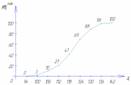 |  |
For graphical representation of variation series, the polygon, histogram, cumulative curve and empirical distribution function are most often used.
In table 2.3 (Grouping of the Russian population by average per capita income in April 1994) is presented interval variation series.
It is convenient to analyze distribution series using a graphical image, which allows one to judge the shape of the distribution. A visual representation of the nature of changes in the frequencies of the variation series is given by polygon and histogram.
The polygon is used when depicting discrete variation series.
Let us, for example, graphically depict the distribution of housing stock by type of apartment (Table 2.10).
Table 2.10 - Distribution of the housing stock of the urban area by type of apartment (conditional figures).

Rice. Housing distribution area
Not only the frequency values, but also the frequencies of the variation series can be plotted on the ordinate axes.
The histogram is used to depict an interval variation series. When constructing a histogram, the values of the intervals are plotted on the abscissa axis, and the frequencies are depicted by rectangles built on the corresponding intervals. The height of the columns in the case of equal intervals should be proportional to the frequencies. A histogram is a graph in which a series is depicted as bars adjacent to each other.
Let us graphically depict the interval distribution series given in table. 2.11.
Table 2.11 - Distribution of families by size of living space per person (conditional figures).
| N p/p | Groups of families by size of living space per person | Number of families with a given size of living space | Cumulative number of families |
| 1 | 3 – 5 | 10 | 10 |
| 2 | 5 – 7 | 20 | 30 |
| 3 | 7 – 9 | 40 | 70 |
| 4 | 9 – 11 | 30 | 100 |
| 5 | 11 – 13 | 15 | 115 |
| TOTAL | 115 | ---- | |

Rice. 2.2. Histogram of the distribution of families by the size of living space per person
Using the data of the accumulated series (Table 2.11), we construct cumulate distribution.

Rice. 2.3. Cumulative distribution of families by size of living space per person
The representation of a variation series in the form of a cumulate is especially effective for variation series whose frequencies are expressed as fractions or percentages of the sum of the series frequencies.
If we change the axes when graphically depicting a variation series in the form of cumulates, then we get ogiva. In Fig. 2.4 shows an ogive constructed on the basis of the data in Table. 2.11.
A histogram can be converted into a distribution polygon by finding the midpoints of the sides of the rectangles and then connecting these points with straight lines. The resulting distribution polygon is shown in Fig. 2.2 with a dotted line.
When constructing a histogram of the distribution of a variation series with unequal intervals, it is not the frequencies that are plotted along the ordinate axis, but the density of the distribution of the characteristic in the corresponding intervals.
The distribution density is the frequency calculated per unit interval width, i.e. how many units in each group are per unit of interval value. An example of calculating the distribution density is presented in table. 2.12.
Table 2.12 - Distribution of enterprises by number of employees (conditional figures)
| N p/p | Groups of enterprises by number of employees, people. | Number of enterprises | Interval size, people. | Distribution density |
| A | 1 | 2 | 3=1/2 | |
| 1 | Up to 20 | 15 | 20 | 0,75 |
| 2 | 20 – 80 | 27 | 60 | 0,25 |
| 3 | 80 – 150 | 35 | 70 | 0,5 |
| 4 | 150 – 300 | 60 | 150 | 0,4 |
| 5 | 300 – 500 | 10 | 200 | 0,05 |
| TOTAL | 147 | ---- | ---- |
Can also be used for graphical representation of variation series cumulative curve. Using a cumulate (sum curve), a series of accumulated frequencies is depicted. Cumulative frequencies are determined by sequentially summing frequencies across groups and show how many units in the population have attribute values no greater than the value under consideration.

Rice. 2.4. Ogive of distribution of families by the size of living space per person
When constructing the cumulates of an interval variation series, variants of the series are plotted along the abscissa axis, and accumulated frequencies are plotted along the ordinate axis.
Variational are called distribution series constructed on a quantitative basis. The values of quantitative characteristics in individual units of the population are not constant and differ more or less from each other.
Variation- fluctuation, changeability of the value of a characteristic among units of the population. Individual numerical values of a characteristic found in the population being studied are called options values. The insufficiency of the average value to fully characterize the population forces us to supplement the average values with indicators that allow us to assess the typicality of these averages by measuring the variability (variation) of the characteristic being studied.
The presence of variation is due to the influence of a large number of factors on the formation of the level of the trait. These factors act with unequal strength and in different directions. Variation indices are used to describe the measure of trait variability.
Objectives of statistical study of variation:
- 1) study of the nature and degree of variation of characteristics in individual units of the population;
- 2) determining the role of individual factors or their groups in the variation of certain characteristics of the population.
In statistics, special methods for studying variation are used, based on the use of a system of indicators, With by which variation is measured.
Research on variation is important. Measuring variations is necessary when conducting sample observation, correlation and variance analysis, etc. Ermolaev O.Yu. Mathematical statistics for psychologists: Textbook [Text]/ O.Yu. Ermolaev. - M.: Flint Publishing House of the Moscow Psychological and Social Institute, 2012. - 335 p.
By the degree of variation one can judge the homogeneity of the population, the stability of individual values of characteristics and the typicality of the average. On their basis, indicators of the closeness of the relationship between characteristics and indicators for assessing the accuracy of sample observation are developed.
A distinction is made between variation in space and variation in time.
Variation in space is understood as the fluctuation of attribute values among population units representing individual territories. Time variation refers to changes in the values of a characteristic over different periods of time.
To study variation in distribution rows, all variants of attribute values are arranged in ascending or descending order. This process is called series ranking.
The simplest signs of variation are minimum and maximum- the smallest and largest value of the attribute in the aggregate. The number of repetitions of individual variants of feature values is called repetition frequency (fi). It is convenient to replace frequencies with frequencies - wi. Frequency is a relative indicator of frequency, which can be expressed in fractions of a unit or as a percentage and allows you to compare variation series with different numbers of observations. Expressed by the formula:
where Xmax, Xmin are the maximum and minimum values of the characteristic in the aggregate; n - number of groups.
To measure the variation of a trait, various absolute and relative indicators are used. Absolute indicators of variation include the range of variation, average linear deviation, dispersion, and standard deviation. Relative indicators of oscillation include the coefficient of oscillation, relative linear deviation, and coefficient of variation.
An example of finding a variation series
Exercise. For this sample:
- a) Find the variation series;
- b) Construct the distribution function;
No.=42. Sample elements:
1 5 1 8 1 3 9 4 7 3 7 8 7 3 2 3 5 3 8 3 5 2 8 3 7 9 5 8 8 1 2 2 5 1 6 1 7 6 7 7 6 2
Solution.
- a) construction of a ranked variation series:
- 1 1 1 1 1 1 2 2 2 2 2 3 3 3 3 3 3 3 4 5 5 5 5 5 6 6 6 7 7 7 7 7 7 7 8 8 8 8 8 8 9 9
- b) construction of a discrete variation series.
Let's calculate the number of groups in the variation series using the Sturgess formula:
Let's take the number of groups to be 7.
Knowing the number of groups, we calculate the size of the interval:
For the convenience of constructing the table, we will take the number of groups equal to 8, the interval will be 1.
Rice. 1 The volume of sales of goods by a store for a certain period of time
The grouping method also allows you to measure variation(variability, fluctuation) of signs. When the number of units in a population is relatively small, variation is measured based on the ranked number of units that make up the population. The series is called ranked, if the units are arranged in ascending (descending) order of the characteristic.
However, ranked series are quite indicative when a comparative characteristic of variation is needed. In addition, in many cases we have to deal with statistical populations consisting of a large number of units, which are practically difficult to represent in the form of a specific series. In this regard, for an initial general acquaintance with statistical data and especially to facilitate the study of variation in characteristics, the phenomena and processes under study are usually combined into groups, and the grouping results are presented in the form of group tables.
If a group table has only two columns - groups according to a selected characteristic (options) and the number of groups (frequency or frequency), it is called near distribution.
Distribution range - the simplest type of structural grouping based on one characteristic, displayed in a group table with two columns containing variants and frequencies of the characteristic. In many cases, with such a structural grouping, i.e. With the compilation of distribution series, the study of the initial statistical material begins.
A structural grouping in the form of a distribution series can be turned into a genuine structural grouping if the selected groups are characterized not only by frequencies, but also by other statistical indicators. The main purpose of distribution series is to study the variation of characteristics. The theory of distribution series is developed in detail by mathematical statistics.
The distribution series are divided into attributive(grouping according to attributive characteristics, for example, dividing the population by gender, nationality, marital status, etc.) and variational(grouping by quantitative characteristics).
Variation series is a group table that contains two columns: grouping of units according to one quantitative characteristic and the number of units in each group. The intervals in the variation series are usually formed equal and closed. The variation series is the following grouping of the Russian population by average per capita monetary income (Table 3.10).
Table 3.10
Distribution of the population of Russia by average per capita income in 2004-2009.
|
Population groups by average per capita cash income, rub./month |
Population in the group, % of the total |
|||||
|
8 000,1-10 000,0 |
||||||
|
10 000,1-15 000,0 |
||||||
|
15 000,1-25 000,0 |
||||||
|
Over 25,000.0 |
||||||
|
Whole population |
||||||
Variation series, in turn, are divided into discrete and interval. Discrete variation series combine variants of discrete characteristics that vary within narrow limits. An example of a discrete variation series is the distribution of Russian families by the number of children they have.
Interval Variation series combine variants of either continuous characteristics or discrete characteristics varying over a wide range. Interval is the variation series of the distribution of the Russian population according to the value of average per capita monetary income.
Discrete variation series are not used very often in practice. Meanwhile, compiling them is not difficult, since the composition of the groups is determined by the specific variants that the studied grouping characteristics actually have.
Interval variation series are more widespread. When compiling them, a difficult question arises about the number of groups, as well as the size of the intervals that should be established.
The principles for solving this issue are set out in the chapter on the methodology for constructing statistical groupings (see paragraph 3.3).
Variation series are a means of collapsing or compressing diverse information into a compact form; from them one can make a fairly clear judgment about the nature of the variation, and study the differences in the characteristics of the phenomena included in the set under study. But the most important significance of variation series is that on their basis the special generalizing characteristics of variation are calculated (see Chapter 7).
Variation determines differences in the values of a characteristic among different units of a given population at the same period (point in time). Variation is caused by different conditions of existence of different units of the population. For example, even twins in the course of their lives acquire differences in height, weight, as well as in such characteristics as level of education, income, number of children, etc.
Variation arises as a result of the fact that the values of the attribute themselves are formed under the total influence of various conditions, which are combined in different ways in each individual case. Thus, the value of any option is objective.
Variation is characteristic to all phenomena of nature and society, without exception, except for the legally established normative meanings of individual social characteristics. Studies of variation in statistics are of great importance; they help to understand the essence of the phenomenon being studied. Finding variation, finding out its causes, identifying the influence of individual factors provide important information for the implementation of scientifically based management decisions.
The average value gives a generalized characteristic of the characteristic of the population, but it does not reveal its structure. The average value does not show how the variants of the averaged characteristic are located around it, whether they are distributed near the average or deviate from it. The average in two populations may be the same, but in one version all individual values differ from it insignificantly, and in the other, these differences are large, i.e. in the first case the variation of the characteristic is small, and in the second it is large; this is very important for characterizing the significance of the average value.
In order for the head of an organization, a manager, or a researcher to study variation and manage it, statistics have developed special methods for studying variation (a system of indicators). With their help, variation is found and its properties are characterized. Variation indicators include : range of variation, average linear deviation, coefficient of variation.
Variation series and its forms
Variation series- this is an ordered distribution of units of a population, often according to increasing (less often decreasing) values of a characteristic and counting the number of units with a particular value of the characteristic. When the number of population units is large, the ranked series becomes cumbersome and its construction takes a long time. In such a situation, a variation series is constructed by grouping population units according to the values of the characteristic being studied.
There are the following variation series forms :
- Ranked series represents a list of individual units of the population in ascending (descending) order of the characteristic being studied.
- Discrete variation series - this is a table consisting of two lines or graphs: specific values of the varying characteristic x and the number of units of the population with a given value f - the frequency characteristic. It is constructed when the attribute takes on the largest number of values.
- Interval series.
The range of variation is determined as the absolute value of the difference between the maximum and minimum values (variants) of the characteristic:
The range of variation shows only extreme deviations of the characteristic and does not reflect individual deviations of all options in the series. It characterizes the limits of change in a varying characteristic and is dependent on fluctuations of two extreme options and is absolutely not related to the frequencies in the variation series, i.e., to the nature of the distribution, which gives this value a random character. To analyze variation, you need an indicator that reflects all fluctuations in the variation characteristic and gives a general characteristic. The simplest indicator of this type is the average linear deviation.
(definition of a variation series; components of a variation series; three forms of a variation series; feasibility of constructing an interval series; conclusions that can be drawn from the constructed series)
A variation series is the sequence of all sample elements arranged in non-decreasing order. Identical elements are repeated
Variational series are series built on a quantitative basis.
Variational distribution series consist of two elements: options and frequencies:
Variants are numerical values of a quantitative characteristic in a variational distribution series. They can be positive and negative, absolute and relative. So, when grouping enterprises according to the results of economic activity, the positive options are profit, and the negative numbers are loss.
Frequencies are the numbers of individual variants or each group of a variation series, i.e. These are numbers showing how often certain options occur in a distribution series. The sum of all frequencies is called the volume of the population and is determined by the number of elements of the entire population.
Frequencies are frequencies expressed as relative values (fractions of units or percentages). The sum of the frequencies is equal to one or 100%. Replacing frequencies with frequencies allows one to compare variation series with different numbers of observations.
There are three forms of variation series: ranked series, discrete series and interval series.
A ranked series is the distribution of individual units of a population in ascending or descending order of the characteristic being studied. Ranking allows you to easily divide quantitative data into groups, immediately detect the smallest and largest values of a characteristic, and highlight the values that are most often repeated.
Other forms of variation series are group tables compiled according to the nature of variation in the values of the characteristic being studied. According to the nature of variation, discrete (discontinuous) and continuous characteristics are distinguished.
A discrete series is a variational series, the construction of which is based on characteristics with discontinuous change (discrete characteristics). The latter include the tariff category, the number of children in the family, the number of employees in the enterprise, etc. These features can only take a finite number of specific values.
A discrete variation series represents a table that consists of two columns. The first column indicates the specific value of the attribute, and the second column indicates the number of units in the population with a specific value of the attribute.
If a characteristic has a continuous change (amount of income, length of service, cost of fixed assets of an enterprise, etc., which can take on any values within certain limits), then for this characteristic it is necessary to build an interval variation series.
The group table here also has two columns. The first indicates the value of the attribute in the interval “from - to” (options), the second indicates the number of units included in the interval (frequency).
Frequency (repetition frequency) - the number of repetitions of a particular variant of attribute values, is denoted fi, and the sum of frequencies equal to the volume of the population under study is denoted
Where k is the number of options for attribute values
Very often, the table is supplemented with a column in which the accumulated frequencies S are calculated, which show how many units in the population have a characteristic value no greater than this value.
A discrete variational distribution series is a series in which groups are composed according to a characteristic that changes discretely and takes only integer values.
An interval variational distribution series is a series in which the grouping characteristic that forms the basis of the grouping can take on any values, including fractional ones, in a certain interval.
An interval variation series is an ordered set of intervals of varying the values of a random variable with the corresponding frequencies or frequencies of occurrences of the value in each of them.
It is advisable to construct an interval distribution series, first of all, with a continuous variation of a characteristic, and also if a discrete variation manifests itself over a wide range, i.e. the number of variants of a discrete characteristic is quite large.
Several conclusions can already be drawn from this series. For example, the middle element of a variation series (median) can be an estimate of the most probable measurement result. The first and last element of the variation series (i.e., the minimum and maximum element of the sample) show the spread of the sample elements. Sometimes, if the first or last element is very different from the rest of the sample, they are excluded from the measurement results, considering that these values were obtained as a result of some kind of gross failure, for example, technology.