Rules for entering functions:
For example, x 1 2 +x 1 x 2, write as x1^2+x1*x2Generates search directions, in to a greater extent corresponding to the geometry of the function being minimized.
Definition . Two n-dimensional vectors x and y are called conjugated with respect to matrix A (or A-conjugate), if dot product(x, Aу) = 0 . Here A is a symmetric positive definite matrix of size n x n.
Scheme of the conjugate gradient method algorithm
Set k=0.Ш. 1 Let x 0 be the starting point; ,
d 0 =-g 0 ; k=0.
Sh. 2 Determine x k +1 =x k +λ k d k, where
 .
.Then d k+1 =-g k+1 +β k d k ,
 ,
,β k is found from the condition d k +1 Ad k =0 (conjugate with respect to matrix A).
Sh. 3 Put k=k+1 → Sh. 2.
The criterion for stopping a one-dimensional search along each direction d k is written as:
Values
Fletcher-Reeves method
Fletcher-Reeves Method Strategy consists in constructing a sequence of points (x k ), k=0, 1, 2, ... such that f(x k +1)< f(x k), k=0, 1, 2, ...The points of the sequence (x k) are calculated according to the rule:
x k +1 =x k -t k d k , k = 0, 1, 2,…
d k = ▽f(x k) + b k -1 ▽f(x k -1)

The step size is selected from the condition of the minimum of the function f(x) over t in the direction of movement, i.e., as a result of solving the one-dimensional minimization problem:
f(x k -t k d k) → min (t k >0)
In case quadratic function f(x)= (x, Hx) + (b, x) + and the directions d k, d k -1 will be H-conjugate, i.e. (d k , Hd k -1)=0
Moreover, at the points of the sequence (x k) function gradients f(x) are mutually perpendicular, i.e. (▽f(x k +1),▽f(x k))=0, k =0, 1, 2…
When minimizing non-quadratic functions, the Fletcher-Reeves method is not finite. For non-quadratic functions, the following modification of the Fletcher-Reeves method (Polak-Ribière method) is used, when the value b k -1 is calculated as follows:

Here I is a set of indices: I = (0, n, 2n, 3n, ...), i.e. the Polak-Ribière method involves the use of the fastest iteration gradient descent every n steps, replacing x 0 with x n +1.
The construction of the sequence(x k) ends at the point for which |▽f(x k)|<ε.
The geometric meaning of the conjugate gradient method is as follows. From a given starting point x 0 descent is carried out in the direction d 0 = ▽f(x 0). At the point x 1 the gradient vector ▽f(x 1) is determined. Since x 1 is the minimum point of the function in the direction d 0, then ▽f(x 1) orthogonal to the vector d 0 . Then the vector d 1 is found, H-conjugate to d 0 . Next, the minimum of the function is found along the direction d 1, etc.

Fletcher-Reeves method algorithm
Initial stage.Set x 0 , ε > 0.
Find the gradient of a function in arbitrary point

k=0.
Main stage
Step 1. Calculate ▽f(x k)
Step 2. Check the fulfillment of the stopping criterion |▽f(x k)|< ε
a) if the criterion is met, the calculation is completed, x * =x k
b) if the criterion is not met, then go to step 3 if k=0, otherwise go to step 4.
Step 3. Determine d 0 = ▽f(x 0)
Step 4. Determine or in the case of a non-quadratic function

Step 5. Determine d k = ▽f(x k) + b k -1 ▽f(x k -1)
Step 6. Calculate the step size t k from the condition f(x k - t k d k) → min (t k >0)
Step 7. Calculate x k+1 =x k -t k d k
Step 8. Set k= k +1 and go to step 1.
Convergence of the method
Theorem 1. If the quadratic function f(x) = (x, Hx) + (b, x) + a with a non-negative definite matrix H reaches its minimum value on R n, then the Fletcher-Reeves method ensures that the minimum point is found in no more than n steps.Theorem 2. Let the function f(x) be differentiable and bounded from below on R m, and its gradient satisfies the Lipschitz condition. Then, for an arbitrary starting point, for the Polac-Ribière method we have
Theorem 2 guarantees the convergence of the sequence (x k ) to stationary point x * , where ▽f(x *)=0. Therefore, the found point x * needs additional research for its classification. The Polak-Ribière method guarantees the convergence of the sequence (x k ) to the minimum point only for highly convex functions.
The convergence rate estimate was obtained only for strongly convex functions, in this case the sequence (x k) converges to the minimum point of the function f(x) with the speed: |x k+n – x*| ≤ C|x k – x*|, k = (0, n, 2, …)
Example. Find the minimum of the function using the conjugate gradient method: f(X) = 2x 1 2 +2x 2 2 +2x 1 x 2 +20x 1 +10x 2 +10.
Solution. As the search direction, select the gradient vector at the current point:
|
Newton's method and the quasi-Newton methods discussed in the previous paragraph are very effective as a means of solving unconstrained minimization problems. However, they present quite high demands to the amount of computer memory used. This is due to the fact that choosing a search direction requires solving systems linear equations, as well as with the emerging need to store matrices of the type Therefore, for large ones, the use of these methods may be impossible. To a significant extent, conjugate direction methods are freed from this drawback.
1. The concept of conjugate direction methods.
Consider the problem of minimizing the quadratic function
![]()
with a symmetric positive definite matrix A Recall that its solution requires one step of the Newton method and no more than steps of the quasi-Newton method. Conjugate direction methods also allow you to find the minimum point of the function (10.33) in no more than steps. This can be achieved through a special selection of search directions.
We will say that nonzero vectors are mutually conjugate (with respect to matrix A) if for all
By the method of conjugate directions for minimizing the quadratic function (10.33) we mean the method
in which the directions are mutually conjugate, and the steps

are obtained as a solution to one-dimensional minimization problems:
Theorem 10.4. The conjugate directions method allows you to find the minimum point of the quadratic function (10 33) in no more than steps.
Conjugate directions methods differ from one another in the way conjugate directions are constructed. The most famous among them is the conjugate gradient method.
2. Conjugate gradient method.
In this method, directions build a rule
![]()
Since the first step of this method coincides with the step of the steepest descent method. It can be shown (we will not do this) that the directions (10.34) are indeed
conjugate with respect to matrix A. Moreover, the gradients turn out to be mutually orthogonal.
Example 10.5. Let's use the conjugate gradient method to minimize the quadratic function - from Example 10.1. Let's write it in the form where
![]()
Let's take the initial approximation
The 1st step of the method coincides with the first step of the steepest descent method. Therefore (see example 10.1)
2nd step. Let's calculate

Since the solution turned out to be found in two steps.
3. Conjugate gradient method for minimizing non-quadratic functions.
In order for this method to be applied to minimize an arbitrary smooth function formula (10.35) for calculating the coefficient is converted to the form
![]()
or to the view
![]()
The advantage of formulas (10 36), (10.37) is that they do not explicitly contain matrix A.
The function is minimized by the conjugate gradient method in accordance with the formulas

The coefficients are calculated using one of the formulas (10.36), (10.37).
The iterative process here no longer ends after finite number steps, and the directions are not, generally speaking, conjugate with respect to some matrix.
One-dimensional minimization problems (10.40) have to be solved numerically. We also note that often in the conjugate gradient method the coefficient is not calculated using formulas (10.36), (10.37), but is assumed equal to zero. In this case, the next step is actually carried out using the steepest descent method. This “updating” of the method allows us to reduce the influence of computational error.
For a strongly convex smooth function for some additional conditions The conjugate gradient method has a high superlinear convergence rate. At the same time, its labor intensity is low and is comparable to the complexity of the steepest descent method. As computational practice shows, it is slightly inferior in efficiency to quasi-Newton methods, but places significantly lower demands on the computer memory used. In the case where the problem of minimizing a function with very a large number variables, the conjugate gradient method appears to be the only suitable universal method.
Computational experiments to evaluate the effectiveness of a parallel version of the upper relaxation method were carried out under the conditions specified in the introduction. In order to form a symmetric positive definite matrix, the elements of the submatrix were generated in the range from 0 to 1, the values of the elements of the submatrix were obtained from the symmetry of the matrices and , and the elements on the main diagonal (submatrix ) were generated in the range from to , where is the size of the matrix.
As a stopping criterion, we used the stopping criterion for accuracy (7.51) with the parameter a iteration parameter . In all experiments, the method found a solution with the required accuracy in 11 iterations. As for previous experiments, we will fix the acceleration in comparison with parallel program, running in one thread.
| n | 1 stream | Parallel algorithm | |||||||
| 2 streams | 4 streams | 6 streams | 8 streams | ||||||
| T | S | T | S | T | S | T | S | ||
| 2500 | 0,73 | 0,47 | 1,57 | 0,30 | 2,48 | 0,25 | 2,93 | 0,22 | 3,35 |
| 5000 | 3,25 | 2,11 | 1,54 | 1,22 | 2,67 | 0,98 | 3,30 | 0,80 | 4,08 |
| 7500 | 7,72 | 5,05 | 1,53 | 3,18 | 2,43 | 2,36 | 3,28 | 1,84 | 4,19 |
| 10000 | 14,60 | 9,77 | 1,50 | 5,94 | 2,46 | 4,52 | 3,23 | 3,56 | 4,10 |
| 12500 | 25,54 | 17,63 | 1,45 | 10,44 | 2,45 | 7,35 | 3,48 | 5,79 | 4,41 |
| 15000 | 38,64 | 26,36 | 1,47 | 15,32 | 2,52 | 10,84 | 3,56 | 8,50 | 4,54 |

Rice. 7.50.
Experiments demonstrate good acceleration (about 4 on 8 threads).
Conjugate gradient method
Consider the system of linear equations (7.49) with a symmetric, positive definite matrix of size . Basis conjugate gradient method is next property: solving the system of linear equations (7.49) with a symmetric positive definite matrix is equivalent to solving the problem of minimizing the function
Goes to zero. Thus, the solution to system (7.49) can be sought as a solution to the unconditional minimization problem (7.56).
Sequential algorithm
In order to solve the minimization problem (7.56), the following iterative process is organized.
The preparatory step () is determined by the formulas
Where is an arbitrary initial approximation; and the coefficient is calculated as

) are determined by the formulas
Here is the discrepancy of the th approximation, the coefficient is found from the conjugacy condition
![]()
Directions and ; is a solution to the problem of minimizing a function in the direction
Analysis of the calculation formulas of the method shows that they include two operations of multiplying a matrix by a vector, four operations of a scalar product and five operations on vectors. However, at each iteration, it is enough to calculate the product once and then use the stored result. Total quantity the number of operations performed in one iteration is
![]()
Thus, performing iterations of the method will require
| (7.58) |
Operations. It can be shown that to find an exact solution to a system of linear equations with a positive definite symmetric matrix, it is necessary to perform no more than n iterations, thus the complexity of the algorithm for finding an exact solution is of the order of . However, due to rounding errors this process usually considered as iterative, the process ends either when the usual stopping condition (7.51) is satisfied, or when the condition of smallness of the relative norm of the residual is satisfied
![]()
Organization of parallel computing
When developing a parallel version of the conjugate gradient method for solving systems of linear equations, first of all, it should be taken into account that the iterations of the method are carried out sequentially and, thus, the most appropriate approach is to parallelize the calculations implemented during the iterations.
Analysis of the sequential algorithm shows that the main costs at the th iteration consist in multiplying the matrix by the vectors and . As a result, well-known methods can be used to organize parallel computations parallel multiplication matrices per vector.
Additional calculations of a lower order of complexity are various vector processing operations (scalar product, addition and subtraction, multiplication by a scalar). The organization of such calculations, of course, must be consistent with the chosen in a parallel way performing the operation of multiplying a matrix by a vector.
For further analysis of the efficiency of the resulting parallel calculations, we will choose a parallel algorithm of matrix-vector multiplication with strip horizontal division of the matrix. In this case, operations on vectors, which are less computationally intensive, will also be performed in multi-threaded mode.
Computational effort sequential method conjugate gradients is determined by relation (7.58). Let's determine the execution time parallel implementation conjugate gradient method. The computational complexity of the parallel operation of multiplying a matrix by a vector when using a strip horizontal matrix partitioning scheme is
Where is the length of the vector, is the number of threads, and is the overhead for creating and closing a parallel section.
All other operations on vectors (dot product, addition, multiplication by a constant) can be performed in single-threaded mode, because are not decisive in the overall complexity of the method. Therefore, the overall computational complexity of the parallel version of the conjugate gradient method can be estimated as

Where is the number of iterations of the method.
Results of computational experiments
Computational experiments to evaluate the effectiveness of a parallel version of the conjugate gradient method for solving systems of linear equations with a symmetric positive definite matrix were carried out under the conditions specified in the introduction. Elements on the main diagonal of the matrix ) were generated in the range from to , where is the size of the matrix, the remaining elements were generated symmetrically in the range from 0 to 1. The stopping criterion for accuracy (7.51) with the parameter was used as a stopping criterion
The results of computational experiments are given in Table 7.21 (the operating time of the algorithms is indicated in seconds).
Method of steepest descent
When using the steepest descent method at each iteration, the step size A k
is selected from the minimum condition of the function f(x) in the direction of descent, i.e.
f(x[k]-a k f"(x[k]))
= f(x[k] -af"(x[k]))
.
This condition means that movement along the antigradient occurs as long as the value of the function f(x) decreases. WITH mathematical point view at each iteration it is necessary to solve the problem of one-dimensional minimization according to A functions
j (a) = f(x[k]-af"(x[k])) .
The algorithm of the steepest descent method is as follows.
1. Set the coordinates of the starting point X.
2. At the point X[k], k = 0, 1, 2, ... calculates the gradient value f"(x[k]) .
3. The step size is determined a k , by one-dimensional minimization over A functions j (a) = f(x[k]-af"(x[k])).
4. The coordinates of the point are determined X[k+ 1]:
X i [k+ 1]= x i [k]- A k f" i (X[k]), i = 1,..., p.
5. The conditions for stopping the steration process are checked. If they are fulfilled, then the calculations stop. Otherwise, go to step 1.
In the method under consideration, the direction of movement from the point X[k] touches the level line at the point x[k+ 1] (Fig. 2.9). The descent trajectory is zigzag, with adjacent zigzag links orthogonal to each other. Indeed, a step a k is chosen by minimizing by A functions q (a) = f(x[k] -af"(x[k])) . Prerequisite minimum function d j (a)/da = 0. Having calculated the derivative complex function, we obtain the condition for the orthogonality of the vectors of descent directions at neighboring points:
d j (a)/da = -f"(x[k+ 1]f"(x[k]) = 0.
Gradient methods converge to a minimum with high speed(at speed geometric progression) for smooth convex functions. Such functions have the greatest M and least m eigenvalues of the matrix of second derivatives (Hessian matrix)

differ little from each other, i.e. matrix N(x) well conditioned. Let us remind you that eigenvalues l i, i =1, …, n, the matrices are the roots of the characteristic equation

However, in practice, as a rule, the functions being minimized have ill-conditioned matrices of second derivatives (t/m<< 1). The values of such functions along some directions change much faster (sometimes by several orders of magnitude) than in other directions. Their level surfaces in the simplest case are strongly elongated, and in more complex cases they bend and appear as ravines. Functions with such properties are called gully. The direction of the antigradient of these functions (see Fig. 2.10) deviates significantly from the direction to the minimum point, which leads to a slowdown in the speed of convergence.
Conjugate gradient method
The gradient methods discussed above find the minimum point of a function in the general case only in an infinite number of iterations. The conjugate gradient method generates search directions that are more consistent with the geometry of the function being minimized. This significantly increases the speed of their convergence and allows, for example, to minimize the quadratic function
f(x) = (x, Hx) + (b, x) + a
with a symmetric positive definite matrix N in a finite number of steps p, equal to the number of function variables. Any smooth function in the vicinity of the minimum point can be well approximated by a quadratic function, therefore conjugate gradient methods are successfully used to minimize non-quadratic functions. In this case, they cease to be finite and become iterative.
By definition, two n-dimensional vector X And at called conjugated relative to the matrix H(or H-conjugate), if the scalar product (x, Well) = 0. Here N - symmetric positive definite matrix of size n X p.
One of the most significant problems in conjugate gradient methods is the problem of efficiently constructing directions. The Fletcher-Reeves method solves this problem by transforming the antigradient at each step -f(x[k]) in the direction p[k], H-conjugate with previously found directions r, r, ..., r[k-1]. Let us first consider this method in relation to the problem of minimizing a quadratic function.
Directions r[k] is calculated using the formulas:
p[k] = -f"(x[k]) +b k-1 p[k-l], k>= 1;
p = -f"(x) .
b values k-1 are chosen so that the directions p[k], r[k-1] were H-conjugate:
(p[k], HP[k- 1])= 0.
As a result, for the quadratic function
the iterative minimization process has the form
x[k+l] =x[k]+a k p[k],
Where r[k] - direction of descent to k- m step; A k - step size. The latter is selected from the minimum condition of the function f(x) By A in the direction of movement, i.e. as a result of solving the one-dimensional minimization problem:
f(x[k] + A k r[k]) = f(x[k] + ar [k]) .
For a quadratic function
The algorithm of the Fletcher-Reeves conjugate gradient method is as follows.
1. At the point X calculated p = -f"(x) .
2. On k- m step, using the above formulas, the step is determined A k . and period X[k+ 1].
3. Values are calculated f(x[k+1]) And f"(x[k+1]) .
4. If f"(x) = 0, then point X[k+1] is the minimum point of the function f(x). Otherwise, a new direction is determined p[k+l] from the relation
and the transition to the next iteration is carried out. This procedure will find the minimum of a quadratic function in no more than n steps. When minimizing non-quadratic functions, the Fletcher-Reeves method becomes iterative from finite. In this case, after (p+ 1)th iteration of procedure 1-4 are repeated cyclically with replacement X on X[n+1] , and the calculations end at, where is a given number. In this case, the following modification of the method is used:
x[k+l] = x[k]+a k p[k],
p[k] = -f"(x[k])+ b k- 1 p[k-l], k>= 1;
p= -f"( x);
f(x[k] + a k p[k]) = f(x[k] +ap[k];

Here I- many indexes: I= (0, n, 2 p, salary, ...), i.e. the method is updated every n steps.
The geometric meaning of the conjugate gradient method is as follows (Fig. 2.11). From a given starting point X descent is carried out in the direction r = -f"(x). At the point X the gradient vector is determined f"(x). Because X is the minimum point of the function in the direction r, That f"(x) orthogonal to vector r. Then the vector is found r , H-conjugate to r. Next, we find the minimum of the function along the direction r etc.

Rice. 2.11 .
Conjugate direction methods are among the most effective for solving minimization problems. However, it should be noted that they are sensitive to errors that occur during the counting process. At large number variables, the error may increase so much that the process will have to be repeated even for a quadratic function, i.e. the process for it does not always fit into n steps.
Gradient methods based only on gradient calculation R(x), are first order methods, since on the step interval they replace the nonlinear function R(x) linear.
Second-order methods that use not only the first, but also the second derivatives of R(x) at the current point. However, these methods have their own difficult to solve problems - the calculation of second derivatives at a point, and furthermore, far from the optimum, the matrix of second derivatives can be poorly conditioned.
The conjugate gradient method is an attempt to combine the advantages of first- and second-order methods while eliminating their disadvantages. On initial stages(far from the optimum) the method behaves like a first-order method, and in the vicinity of the optimum it approaches second-order methods.
The first step is similar to the first step of the steepest descent method, the second and next steps are chosen each time in the direction formed as a linear combination of the gradient vectors at a given point and the previous direction.
The method algorithm can be written as follows (in vector form):
x 1 = x 0 – h grad R(x 0),
x i+1 = x i – h .
The value α can be approximately found from the expression
The algorithm works as follows. From the starting point X 0 looking for min R(x) in the direction of the gradient (using the steepest descent method), then, starting from the found point and further, the search direction min is determined by the second expression. The search for the minimum in the direction can be carried out in any way: you can use the sequential scanning method without adjusting the scanning step when passing the minimum, so the accuracy of achieving the minimum in the direction depends on the step size h.
For a quadratic function R(x) a solution can be found in n steps (p– dimension of the problem). For other functions, the search will be slower, and in some cases may not reach the optimum at all due to strong influence computational errors.
One of the possible trajectories for searching for the minimum of a two-dimensional function using the conjugate gradient method is shown in Fig. 1.
Algorithm of the conjugate gradient method for finding the minimum.
Initial stage. Execution of the gradient method.
Set the initial approximation x 1 0 ,X 2 0 . Determining the value of the criterion R(x 1 0 ,X 2 0). Set k = 0 and go to step 1 of the initial stage.
Step 1.  And
And 
 .
.
Step 2. If the gradient module 
Step 3.
x k+1 = x k – h grad R(x k)).
Step 4. R(x 1 k +1 , X 2 k +1). If R(x 1 k +1 , X 2 k +1)< R(x 1k, X 2 k), then set k = k+1 and go to step 3. If R(x 1 k +1 , X 2 k +1) ≥ R(x 1k, X 2 k), then go to the main stage.
Main stage.
Step 1. Calculate R(x 1 k + g, x 2 k), R(x 1 k – g, x 2 k), R(x 1 k , x 2 k + g), R(x 1 k , x 2 k) . In accordance with the algorithm, from a central or paired sample, calculate the value of partial derivatives  And
And 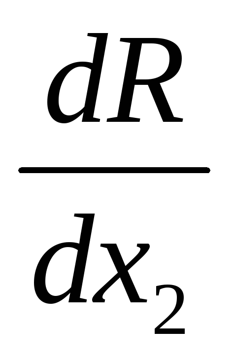 . Calculate the gradient modulus value
  .
.
Step 2. If the gradient module  , then stop the calculation, and consider the point (x 1 k, x 2 k) to be the optimum point. Otherwise, go to step 3.
Step 3. Calculate coefficient α according to the formula:

Step 4. Perform the work step by calculating using the formula
x k+1 = x k – h .
Step 5. Determine the criterion value R(x 1 k +1 , X 2 k +1). Set k = k+1 and go to step 1.
Example.
For comparison, consider the solution to the previous example. We take the first step using the steepest descent method (Table 5).
Table 5
The best point has been found. We calculate the derivatives at this point: dR/ dx 1 = –2.908; dR/ dx 2 =1.600; We calculate the coefficient α, which takes into account the influence of the gradient at the previous point: α = 3.31920 ∙ 3.3192/8.3104 2 =0.160. We take a working step in accordance with the algorithm of the method, we get X 1 = 0,502, X 2 = 1.368. Then everything is repeated in the same way. Below, in the table. 6 shows the current search coordinates for the next steps.
Table 6