Equivalent matrices
As mentioned above, the minor of a matrix of order s is the determinant of a matrix formed from elements of the original matrix located at the intersection of any selected s rows and s columns.
Definition. In a matrix of order mn, a minor of order r is called basic if it is not equal to zero, and all minors of order r+1 and higher are equal to zero or do not exist at all, i.e. r matches the smaller of m or n.
The columns and rows of the matrix on which the basis minor stands are also called basis.
A matrix can have several different basis minors that have the same order.
Definition. The order of the basis minor of a matrix is called the rank of the matrix and is denoted by Rg A.
Very important property elementary matrix transformations is that they do not change the rank of the matrix.
Definition. Matrices obtained as a result of an elementary transformation are called equivalent.
It should be noted that equal matrices and equivalent matrices are completely different concepts.
Theorem. Largest number linearly independent columns in a matrix are equal to the number of linearly independent rows.
Because elementary transformations do not change the rank of the matrix, then the process of finding the rank of the matrix can be significantly simplified.
Example. Determine the rank of the matrix.
2. Example: Determine the rank of the matrix.
If, using elementary transformations, it is not possible to find a matrix equivalent to the original one, but of a smaller size, then finding the rank of the matrix should begin by calculating the minors of the highest possible order. In the above example, these are minors of order 3. If at least one of them is not equal to zero, then the rank of the matrix is equal to the order of this minor.
The theorem on the basis minor.
Theorem. In an arbitrary matrix A, each column (row) is a linear combination of the columns (rows) in which the basis minor is located.
So the rank arbitrary matrix A is equal to maximum number linearly independent rows (columns) in a matrix.
If A is a square matrix and det A = 0, then at least one of the columns is a linear combination of the remaining columns. The same is true for strings. This statement follows from the property linear dependence with the determinant equal to zero.
Solving arbitrary systems of linear equations
As stated above, matrix method and Cramer's method are applicable only to those systems linear equations, in which the number of unknowns is equal to the number of equations. Next, we consider arbitrary systems of linear equations.
Definition. System of m equations with n unknowns in general view is written as follows:

where aij are coefficients and bi are constants. The solutions of the system are n numbers, which, when substituted into the system, turn each of its equations into an identity.
Definition. If a system has at least one solution, then it is called joint. If a system does not have a single solution, then it is called inconsistent.
Definition. A system is called determinate if it has only one solution and indefinite if it has more than one.
Definition. For a system of linear equations the matrix

A = is called the matrix of the system, and the matrix

A*= is called the extended matrix of the system
Definition. If b1, b2, …,bm = 0, then the system is called homogeneous. homogeneous system always joint, because always has a zero solution.
Elementary system transformations
Elementary transformations include:
1) Adding to both sides of one equation the corresponding parts of the other, multiplied by the same number, not equal to zero.
2) Rearranging the equations.
3) Removing from the system equations that are identities for all x.
Kronecker-Kapeli theorem (consistency condition for the system).
(Leopold Kronecker (1823-1891) German mathematician)
Theorem: A system is consistent (has at least one solution) if and only if the rank of the system matrix is equal to the rank of the extended matrix.
Obviously, system (1) can be written in the form.
Let R And S two vector spaces dimensions n And m respectively over the number field K, and let A linear operator displaying R V S. Let's find out how the operator matrix changes A when changing bases in spaces R V S.
Let us choose arbitrary bases in the spaces R V S and denote by and respectively. Then (see linear operators) the vector equality
| (1) |
corresponds to the matrix equality
| (2) |
Where X And at vectors x And y, presented in the form of coordinate columns in bases and, respectively.
Let us now choose in the spaces R And S other bases ![]() And
And ![]() . In the new bases, vector equality (1) will correspond to the matrix equality
. In the new bases, vector equality (1) will correspond to the matrix equality
Then, taking into account (3) and (4), we have
Definition 1. Two rectangular matrices A and B same sizes are said to be equivalent if there exist two square non-singular matrices P And T such that the equality holds
| (7) |
Note that if A-order matrix m×n, That P And T square order matrices m And n, respectively.
From (6) it follows that two matrices corresponding to the same linear operator A for different choices of bases in spaces R And S are equivalent to each other. The converse is also true. If matrix A corresponds to the operator A, and the matrix B is equivalent to the matrix A, then it corresponds to the same linear operator A for other bases in R And S.
Let us find out under what conditions two matrices are equivalent.
Theorem. In order for two matrices of the same size to be equivalent, it is necessary and sufficient that they have the same rank.
Proof. Necessity. Since multiplying a matrix by a square non-singular matrix cannot change the rank of the matrix, then from (7) we have:
Adequacy. Let a linear operator be given A, representing space R V S and let this operator be answered by the matrix A size m×n in bases in R and in S, respectively. Let us denote by r number is linear independent vectors from among Ae 1 , Ae 2 ,..., Aen. Let the first ones be linearly independent r vectors Ae 1 , Ae 2 ,..., Aer. Then the rest n-r vectors are expressed linearly in terms of these vectors:
| Aek = | n | c ijAej, (k=r+1,...n) |
| ∑ | ||
| j= 1 |
Let's define a new basis in space R:
Let's supplement these vectors with some vectors ![]() to base in S.
to base in S.
Then the operator matrix A in new bases ![]() ,
, ![]() according to (9) and (10) will have the following form:
according to (9) and (10) will have the following form:
| (11) |

where in the matrix E" - on the main diagonal they stand r units, and the remaining elements are zero.
Since the matrices A And E" match the same operator A, then they are equivalent to each other. Above we showed that equivalent matrices have the same rank, hence the rank of the original matrix A equals r.
From the above it follows that arbitrary m×n rank matrix r is equivalent to the matrix E" - order m×n. But E" - is uniquely determined by specifying the dimension m×n matrix and its rank r. Therefore, all rectangular matrices of order m×n and rank r are equivalent to the same matrix E" and, therefore, are equivalent to each other.■
Document: I.e. The rank of the matrix is preserved when performing the following operations:
1. Changing the order of lines.
2. Multiplying a matrix by a number other than zero.
3. Transposition.
4. Eliminating a string of zeros.
5. Adding another string to a string, multiplied by an arbitrary number.
The first transformation will leave some minors unchanged, but will change the sign of some to the opposite. The second transformation will also leave some minors unchanged, while others will be multiplied by a number other than zero. The third transformation will preserve all minors. Therefore, when applying these transformations, the rank of the matrix will also be preserved (second definition). Eliminating a zero row cannot change the rank of the matrix, because such a row cannot enter a non-zero minor. Let's consider the fifth transformation.
We will assume that the basis minor Δp is located in the first p rows. Let an arbitrary string b be added to string a, which is one of these strings, multiplied by some number λ. Those. to string a is added a linear combination of strings containing the basis minor. In this case, the basis minor Δp will remain unchanged (and different from 0). Other minors placed in the first p lines also remain unchanged, the same is true for all other minors. That. V in this case the rank (by the second definition) will be preserved. Now consider the minor Ms, which does not have all the rows from among the first p rows (and perhaps it does not have any).
By adding an arbitrary string b to the string ai, multiplied by the number λ, we obtain a new minor Ms‘, and Ms‘=Ms+λ Ms, where
![]()
If s>p, then Ms=Ms=0, because all minors of order greater than p of the original matrix are equal to 0. But then Ms‘=0, and the rank of matrix transformations does not increase. But it could not decrease either, since the basic minor did not undergo any changes. So, the rank of the matrix remains unchanged.
You can also find the information you are interested in in the scientific search engine Otvety.Online. Use the search form:
The first three paragraphs of this chapter are devoted to the doctrine of equivalence of polynomial matrices. On the basis of this, in the next three paragraphs, an analytical theory of elementary divisors is constructed, i.e., a theory of reducing a constant (few-nomial) square matrix to normal form. The last two paragraphs of the chapter give two methods for constructing a transformation matrix.
§ 1. Elementary transformations of a polynomial matrix
Definition 1. A polynomial matrix or -matrix is a rectangular matrix whose elements are polynomials in:
here is the greatest degree of the polynomials.
we can represent a polynomial matrix as a matrix polynomial with respect to , that is, as a polynomial with matrix coefficients:
Let us introduce into consideration the following elementary operations on a polynomial matrix:
1. Multiplying some, for example th, line by a number.
2. Adding to some, for example the th, line another, for example the th, line, previously multiplied by an arbitrary polynomial.
3. Swap any two lines, for example the th and th lines.
We invite the reader to check that operations 1, 2, 3 are equivalent to multiplying a polynomial matrix on the left, respectively, by the following square matrices of order :
 (1)
(1)
i.e., as a result of applying operations 1, 2, 3, the matrix is transformed, respectively, into the matrices , , . Therefore, operations of type 1, 2, 3 are called left elementary operations.
The right elementary operations on a polynomial matrix are defined in a completely similar way (these operations are performed not on the rows, but on the columns of the polynomial matrix) and the corresponding matrices (of order ):

As a result of applying the right elementary operation, the matrix is multiplied on the right by the corresponding matrix.
We will call matrices of type (or, what is the same, type ) elementary matrices.
Determinant any elementary matrix does not depend on and is different from zero. Therefore, for each left (right) elementary operation there is reverse operation, which is also a left (respectively right) elementary operation.
Definition 2. Two polynomial matrices are called 1) left equivalent, 2) right equivalent, 3) equivalent if one of them is obtained from the other by applying, respectively, 1) left elementary operations, 2) right elementary operations, 3) left and right elementary operations.
Let the matrix be obtained from using left elementary operations corresponding to matrices . Then
![]() . (2).
. (2).
Denoting by the product , we write equality (2) in the form
![]() , (3)
, (3)
where , like each of the matrices, has a nonzero constant determinant.
In the next paragraph it will be proven that each square matrix with a constant non-zero determinant can be represented as a product of elementary matrices. Therefore, equality (3) is equivalent to equality (2) and therefore means the left equivalence of the matrices and .
In the case of right equivalence polynomial matrices and instead of equality (3) we will have the equality
![]() , (3")
, (3")
and in the case of (bilateral) equivalence – equality
Here again and are matrices with nonzero and independent determinants.
Thus, Definition 2 can be replaced by an equivalent definition.
Definition 2". Two rectangular matrices and are called 1) left equivalent, 2) right equivalent, 3) equivalent if, respectively
1)
![]() , 2)
, 2) ![]() , 3) ,
, 3) ,
where and are polynomial square matrices with constant and nonzero determinants.
We illustrate all the concepts introduced above with the following important example.
Consider a system of linear homogeneous differential equations-th order with unknown argument functions with constant coefficients:
 (4)
(4)
Mu equation of a new unknown function; the second elementary operation means the introduction of a new unknown function ![]() (instead of ); the third operation means changing places in the equations of terms containing and (i.e.
(instead of ); the third operation means changing places in the equations of terms containing and (i.e. ![]() ).
).
Our immediate goal is to prove that any matrix can be reduced to some standard types. The language of equivalent matrices is useful along this path.
Let it be. We will say that a matrix is l_equivalent (n_equivalent or equivalent) to a matrix and denote (or) if the matrix can be obtained from a matrix using finite number row (column or row and column, respectively) elementary transformations. It is clear that l_equivalent and p_equivalent matrices are equivalent.
First we will show that any matrix can be reduced to special type, called reduced.
Let it be. A non-zero row of this matrix is said to have a reduced form if it contains an element equal to 1 such that all elements of the column other than are equal to zero, . We will call the marked single element of the line the leading element of this line and enclose it in a circle. In other words, a row of a matrix has the reduced form if this matrix contains a column of the form
For example, in the following matrix

the line has the following form, since. Let us pay attention to the fact that in this example, an element also pretends to be the leading element of the line. In the future, if a line of the given type contains several elements that have leading properties, we will select only one of them in an arbitrary manner.
A matrix is said to have a reduced form if each of its non-zero rows has a reduced form. For example, matrix

has the following form.
Proposition 1.3 For any matrix there is an equivalent matrix of the reduced form.
Indeed, if the matrix has the form (1.1) and, then after carrying out elementary transformations in it
we get the matrix

in which the string has the following form.
Secondly, if the row in the matrix was reduced, then after carrying out elementary transformations (1.20) the row of the matrix will be reduced. Indeed, since given, there is a column such that

but then and, consequently, after carrying out transformations (1.20) the column does not change, i.e. . Therefore, the line has the following form.
Now it is clear that by transforming each non-zero row of the matrix in turn in the above manner, after a finite number of steps we will obtain a matrix of the reduced form. Since only row elementary transformations were used to obtain the matrix, it is l_equivalent to a matrix. >
Example 7. Construct a matrix of reduced form, l_equivalent to the matrix