Basic concepts. Theorems of addition and multiplication.
Formulas full probability, Bayes, Bernoulli. Laplace's theorems.
Questions
- Subject of probability theory.
- Types of events.
- Classic definition of probability.
- Statistical definition probabilities.
- Geometric definition probabilities.
- Probability addition theorem Not joint events.
- The probability multiplication theorem is not dependent events.
- Conditional probability.
- Multiplying dependent events.
- Addition of joint events.
- Total probability formula.
- Bayes formula.
13. Binomial, polynomial distribution law.
- Subject of probability theory. Basic concepts.
An event in probability theory is any fact that can occur as a result of some experience (test).
For example: The shooter shoots at the target. A shot is a test, hitting a target is an event. Events are usually designated
A single random event is a consequence of many random causes, which very often cannot be taken into account. However, if we consider mass homogeneous events (observed many times during the experiment under the same conditions), then they turn out to be subject to certain patterns: if you throw a coin in the same conditions a large number of times, you can predict with a small error that the number of occurrences coat of arms will be equal to half the number of throws.
The subject of probability theory is the study of probabilistic patterns of mass homogeneous random events. Methods of probability theory are widely used in the theories of reliability, shooting, automatic control, etc. Probability theory serves as the basis for mathematical and applied statistics, which in turn is used in planning and organizing production, in analyzing technological processes etc.
Definitions.
1. If as a result of the experience the event
a) will always happen, then it is a reliable event,
b) will never happen, then - an impossible event,
c) it may happen, it may not happen, then it is a random (possible) event.
2. Events are called equally possible if there is reason to believe that none of these events has more chances emerge from experience than others.
3. Events and are joint (incompatible), if the occurrence of one of them does not exclude (excludes) the occurrence of the other.
4. A group of events is compatible if at least two events from this group are compatible, otherwise it is incompatible.
5. A group of events is called complete if one of them will definitely occur as a result of the experience.
Example 1. Three shots are fired at the target: Let - hit (miss) on the first shot - on the second shot - on the third shot. Then
a) - a joint group of equally possible events.
b) - a complete group of incompatible events. - an event that is the opposite.
c) - a complete group of events.
Classical and statistical probability
Classic way probability determination is applied to a complete group of equally possible incompatible events.
Each event in this group will be called a case or an elementary outcome. In relation to each event, cases are divided into favorable and unfavorable.
Definition 2. The probability of an event is the quantity
where is the number of cases favorable to the occurrence of the event, is the total number of equally possible this experience cases.
Example 2. Two thrown dice. Let the event - the sum of the dropped points be equal to . Find .
a) Wrong decision. There are only 2 possible cases: and - a complete group of incompatible events. Only one case is favorable, i.e. ![]()
This is a mistake, since they are not equally possible.
b) Total equally possible cases. Favorable cases: prolapse
The weaknesses of the classical definition are:
1. - the number of cases is finite.
2. The result of an experiment very often cannot be represented in the form of a set of elementary events (cases).
3. It is difficult to indicate the reasons for considering cases to be equally possible.
Let a series of tests be carried out.
Definition 3. The relative frequency of an event is the quantity
where is the number of trials in which events appeared and is the total number of trials.
Long-term observations have shown that in various experiences at sufficiently large
Changes little, fluctuating around a certain constant number, which we call statistical probability.
Probability has the following properties:
Algebra of events
7.3.1 Definitions.
8. The sum or union of several events is an event consisting of at least one of them.
9. The product of several events is an event consisting of the joint occurrence of all these events.
From example 1. ![]() - at least one hit with three shots, - a hit with the first and second shots and a miss with the third.
- at least one hit with three shots, - a hit with the first and second shots and a miss with the third.
Exactly one hit.
At least two hits.
10. Two events are called independent (dependent) if the probability of one of them does not depend (depends) on the occurrence or non-occurrence of the other.
11. Several events are called collectively independent if each of them and any linear combination of the remaining events are independent events.
12. Conditional probability ![]() is the probability of an event calculated under the assumption that the event occurred.
is the probability of an event calculated under the assumption that the event occurred.
7.3.2 Probability multiplication theorem.
The probability of the joint occurrence (production) of several events is equal to the product of the probability of one of them by conditional probabilities remaining events calculated under the assumption that all previous events took place
Corollary 1. If - are jointly independent, then
Indeed: since .
Example 3. There are 5 white, 4 black and 3 blue balls in the urn. Each test consists of drawing one ball at random from an urn. What is the probability that on the first test there will be white ball, with the second - a black ball, with the third - a blue ball, if
a) each time the ball returns to the urn.
![]() - in the urn after the first test of balls, 4 of them are white. . From here
- in the urn after the first test of balls, 4 of them are white. . From here
b) the ball does not return to the urn. Then - independent in the aggregate and
7.3.3 Probability addition theorem.
The probability of at least one of the events occurring is equal to
Corollary 2. If the events are pairwise incompatible, then
Indeed in this case
Example 4. Three shots are fired at one target. The probability of a hit on the first shot is , on the second - , on the third - . Find the probability of at least one hit.
Solution. Let there be a hit on the first shot, on the second, on the third, and at least one hit on three shots. Then , where are the joint independent ones in the aggregate. Then
Corollary 3. If pairwise incompatible events form full group, That
Corollary 4. For opposite events
Sometimes when solving problems it is easier to find the probability of the opposite event. For example, in example 4 - a miss with three shots. Since independent in aggregate, and then
As stated above, classic definition probability assumes that all elementary outcomes are equally possible. The equality of the outcomes of the experiment is concluded due to considerations of symmetry. Problems in which symmetry considerations can be used are rare in practice. In many cases it is difficult to provide reasons for believing that all elementary outcomes are equally possible. In this regard, it became necessary to introduce another definition of probability, called statistical. Let us first introduce the concept of relative frequency.
Relative frequency of the event, or frequency, is the ratio of the number of experiments in which this event occurred to the number of all experiments performed. Let us denote the frequency of the event A through W(A), Then
Where n– total number of experiments; m– number of experiments in which the event occurred A.
With a small number of experiments, the frequency of the event is largely random and can vary noticeably from one group of experiments to another. For example, with some ten coin tosses it is quite possible that the coat of arms will appear 2 times (frequency 0.2), with another ten tosses we may well get 8 coats of arms (frequency 0.8). However, with an increase in the number of experiments, the frequency of the event increasingly loses its random character; the random circumstances inherent in each individual experience cancel out in the mass, and the frequency tends to stabilize, approaching with minor fluctuations a certain average constant value. This constant, which is objective numerical characteristic phenomena are considered the probability of a given event.
Statistical definition of probability: probability events name the number around which the frequency values of a given event in different series are grouped large number tests.
The property of frequency stability, repeatedly tested experimentally and confirmed by the experience of mankind, is one of the most characteristic patterns observed in random events. There is a deep connection between the frequency of an event and its probability, which can be expressed as follows: when we evaluate the degree of possibility of an event, we associate this assessment with a greater or lesser frequency of occurrence of similar events in practice.
Geometric probability
 The classic definition of probability assumes that the number elementary outcomes Certainly. In practice, there are experiments for which the set of such outcomes is infinite. In order to overcome this drawback of the classical definition of probability, which is that it is not applicable to tests with an infinite number of outcomes, they introduce geometric probabilities – the probabilities of a point falling into an area.
Let us assume that a quadratable region is given on the plane G, i.e. area having area S G. In the area G contains area g area S g. To the region G A dot is thrown at random. We will assume that the thrown point can fall into some part of the area G with a probability proportional to the area of this part and independent of its shape and location. Let the event A– “the thrown point hits the area g", Then geometric probability this event is determined by the formula:
IN general case The concept of geometric probability is introduced as follows. Let us denote the measure of the area g(length, area, volume) through mes g, and the measure of the area G- through mes G ; let also A– event “a thrown point hits the area g, which is contained in the area G" Probability of hitting the area g points thrown into the area G, is determined by the formula
 .
.
Task. A square is inscribed in a circle. A dot is thrown into the circle at random. What is the probability that the point will fall into the square?
Solution. Let the radius of the circle be R, then the area of the circle is . The diagonal of the square is , then the side of the square is , and the area of the square is . The probability of the desired event is defined as the ratio of the area of the square to the area of the circle, i.e. ![]() .
.
Security questions
1. What is called a test (experience)?
2. What is an event?
3. What event is called a) reliable? b) random? c) impossible?
4. What events are called a) incompatible? b) joint?
5. What events are called opposite? Are they a) incompatible b) compatible or random?
6. What is called a complete group of random events?
7. If the events cannot all happen together as a result of the test, will they be pairwise incompatible?
8. Do events form A and the full group?
9. What elementary outcomes are favorable? this event?
10. What definition of probability is called classical?
11. What are the limits of the probability of any event?
12. Under what conditions does it apply? classical probability?
13. Under what conditions is geometric probability applied?
14. What definition of probability is called geometric?
15. What is the frequency of an event?
16. What definition of probability is called statistical?
1. One letter is selected at random from the letters of the word “conservatory”. Find the probability that this letter is a vowel. Find the probability that it is the letter "o".
2. The letters “o”, “p”, “s”, “t” are written on identical cards. Find the probability that the word “cable” will appear on cards placed randomly in a row.
3. There are 4 women and 3 men in the team. 4 tickets to the theater are raffled off among brigade members. What is the probability that among the ticket holders there will be 2 women and 2 men?
4. Two dice are tossed. Find the probability that the sum of points on both dice is greater than 6.
5. The letters l, m, o, o, t are written on five identical cards. What is the probability that, taking out the cards one at a time, we will get the word “hammer” in the order they appeared?
6. Out of 10 tickets, 2 are winning. What is the probability that among five tickets taken at random, one is winning?
7. What is the probability that in a randomly selected double digit number the numbers are such that their product is equal to zero.
8. A number not exceeding 30 is chosen at random. Find the probability that this number is a divisor of 30.
9. A number not exceeding 30 is chosen at random. Find the probability that this number is a multiple of 3.
10. A number not exceeding 50 is chosen at random. Find the probability that this number is prime.
Indicator rank correlation Kendall, testing the corresponding hypothesis about the significance of the relationship.
2.Classical definition of probability. Properties of probability.
Probability is one of the basic concepts of probability theory. There are several definitions of this concept. Let us give a definition that is called classical. Next we indicate weaknesses this definition and give other definitions that allow us to overcome the shortcomings of the classical definition.
Let's look at an example. Let the urn contain 6 identical, thoroughly mixed balls, and 2 of them are red, 3 are blue and 1 is white. Obviously, the possibility of drawing a colored (i.e., red or blue) ball from an urn at random is greater than the possibility of drawing a white ball. Can this opportunity be quantified? It turns out that it is possible. This number is called the probability of an event (the appearance of a colored ball). Thus, probability is a number that characterizes the degree of possibility of an event occurring.
Let us set ourselves the task of giving quantification the possibility that a ball taken at random is colored. The appearance of a colored ball will be considered as event A. Each of the possible results of the test (the test consists of removing the ball from the urn) will be called elementary outcome (elementary event). We denote elementary outcomes by w 1, w 2, w 3, etc. In our example, the following 6 elementary outcomes are possible: w 1 - a white ball appears; w 2, w 3 - a red ball appeared; w 4, w 5, w 6 - a blue ball appears. It is easy to see that these outcomes form a complete group of pairwise incompatible events (only one ball will appear) and they are equally possible (the ball is drawn at random, the balls are identical and thoroughly mixed).
We will call those elementary outcomes in which the event of interest to us occurs favorable this event. In our example, the following 5 outcomes favor event A (the appearance of a colored ball): w 2, w 3, w 4, w 5, w 6.
Thus, event A is observed if one of the elementary outcomes favoring A occurs in the test, no matter which one; in our example, A is observed if w 2, or w 3, or w 4, or w 5, or w 6 occurs. In this sense, event A is divided into several elementary events (w 2, w 3, w 4, w 5, w 6); an elementary event is not subdivided into other events. This is the difference between event A and an elementary event (an elementary outcome).
The ratio of the number of elementary outcomes favorable to event A to their total number is called the probability of event A and is denoted by P (A). In the example under consideration, there are 6 elementary outcomes; 5 of them favor event A. Consequently, the probability that the taken ball will be colored is equal to P (A) = 5 / 6. This number gives the quantitative assessment of the degree of possibility of the appearance of a colored ball that we wanted to find. Let us now give the definition of probability.
Probability of event A they call the ratio of the number of outcomes favorable to this event to the total number of all equally possible incompatible elementary outcomes that form the complete group. So, the probability of event A is determined by the formula
where m is the number of elementary outcomes favorable to A; n is the number of all possible elementary test outcomes.
Here it is assumed that the elementary outcomes are incompatible, equally possible and form a complete group. The following properties follow from the definition of probability:
With in about s t in about 1. Probability reliable event equal to one.
Indeed, if the event is reliable, then every elementary outcome of the test favors the event. In this case m = n, therefore,
P (A) = m / n = n / n = 1.
S in about with t in about 2. The probability of an impossible event is zero.
Indeed, if an event is impossible, then none of the elementary outcomes of the test favor the event. In this case m = 0, therefore,
P (A) = m / n = 0 / n = 0.
With in about with t in about 3. Probability random event There is positive number, enclosed between zero and one.
Indeed, a random event favors only a part of the total number of elementary outcomes of the test. In this case 0< m < n, значит, 0 < m / n < 1, следовательно,
0 < Р (А) < 1
So, the probability of any event satisfies the double inequality
Remark: Modern rigorous courses in probability theory are built on a set-theoretic basis. Let us limit ourselves to presenting in the language of set theory the concepts discussed above.
Let one and only one of the events w i, (i = 1, 2, ..., n) occur as a result of the test. Events w i are called elementary events (elementary outcomes). It already follows from this that elementary events are pairwise incompatible. The set of all elementary events that can occur in a test is called space of elementary events W, and the elementary events themselves are points of space W.
Event A is identified with a subset (of space W), the elements of which are elementary outcomes favorable to A; event B is a subset of W whose elements are outcomes favorable to B, etc. Thus, the set of all events that can occur in a test is the set of all subsets of W. W itself occurs for any outcome of the test, therefore W is a reliable event; an empty subset of the space W is an impossible event (it does not occur under any outcome of the test).
Note that elementary events are distinguished from all events by the fact that each of them contains only one element W.
Each elementary outcome w i is assigned a positive number p i is the probability of this outcome, and
By definition, the probability P(A) of event A is equal to the sum of the probabilities of elementary outcomes favorable to A. From here it is easy to obtain that the probability of a reliable event is equal to one, an impossible event is equal to zero, and an arbitrary event is between zero and one.
Let's consider an important special case when all outcomes are equally possible. The number of outcomes is n, the sum of the probabilities of all outcomes is equal to one; therefore, the probability of each outcome is 1/n. Let event A be favored by m outcomes. The probability of event A is equal to the sum of the probabilities of outcomes favoring A:
P (A) = 1 / n + 1 / n + .. + 1 / n.
Considering that the number of terms is equal to m, we have
P(A) = m/n.
The classical definition of probability is obtained.
Construction logically full theory probabilities based on axiomatic definition random event and its probability. In the system of axioms proposed by A. N. Kolmogorov, indefinable concepts are elementary event and probability. Here are the axioms that define probability:
1. Each event A is associated with a non-negative real number R(A). This number is called the probability of event A.
2. The probability of a reliable event is equal to one:
3. The probability of the occurrence of at least one of the pairwise incompatible events is equal to the sum of the probabilities of these events.
Based on these axioms, the properties of probabilities and the dependencies between them are derived as theorems.
3.Static determination of probability, relative frequency.
The classical definition does not require experimentation. While real applied problems have infinite number outcomes, and the classical definition in this case cannot provide an answer. Therefore, in such problems we will use static definition probabilities, which is calculated after an experiment or experiment.
Static probability w(A) or relative frequency is the ratio of the number of outcomes favorable for a given event to the total number of tests actually performed.
w(A)=nm
Relative frequency event has stability property:
lim n→∞P(∣ ∣ nm−p∣ ∣ <ε)=1 (свойство устойчивости относительной частоты)
4. Geometric probabilities.
At geometric approach to the definition probabilities an arbitrary set is considered as the space of elementary events finite Lebesgue measure on a line, plane or space. Events are called all kinds of measurable subsets of the set.
Probability of event A is determined by the formula

where denotes Lebesgue measure of the set A. With this definition of events and probabilities, everything A.N. Kolmogorov’s axioms are satisfied.
In specific tasks that boil down to the above probabilistic scheme, the test is interpreted as a random selection of a point in some area, and the event A– how the selected point hits a certain subregion A of the region. In this case, it is required that all points in the region have equal opportunity to be selected. This requirement is usually expressed in words “at random”, “randomly”, etc.
The concept of probability of an event refers to the fundamental concepts of probability theory. Probability is a quantitative measure of the possibility of the occurrence of a random event A. It is denoted by P(A) and has the following properties.
Probability is a positive number ranging from zero to one:
The probability of an impossible event is zero
The probability of a reliable event is equal to one
Classic definition of probability. Let = (1, 2,…, n) be the space of elementary events that describe all possible elementary outcomes and form a complete group of incompatible and equally possible events. Let event A correspond to a subset of m elementary outcomes
these outcomes are called favorable to event A. In the classical definition of probability, it is believed that the probability of any elementary outcome
and the probability of event A favored by m outcomes is equal to
Hence the definition:
The probability of event A is the ratio of the number of outcomes favorable to this event to the total number of all equally possible incompatible elementary outcomes that form the complete group. The probability is given by the formula
where m is the number of elementary outcomes favorable to event A, and is the number of all possible elementary outcomes of the test.
The classical definition of probability makes it possible in some problems to analytically calculate the probability of an event.
Let an experiment be carried out as a result of which certain events may occur. If these events form a complete group of pairwise incompatible and equally possible events, then experience is said to have symmetry of possible outcomes and is reduced to a “scheme of cases.” For experiments that are reduced to a case scheme, the classical probability formula is applicable.
Example 1.13. The lottery draws 1000 tickets, including 5 winning ones. Determine the probability that when purchasing one lottery ticket you will receive a win
The elementary event of this experience is the purchase of a ticket. Each lottery ticket is unique, as it has its own number, and the purchased ticket is not returned. Event A is that the winning ticket is purchased. When buying one of 1000 tickets, all possible outcomes of this experience will be = 1000, the outcomes form a complete group of incompatible events. The number of outcomes favorable to event A will be equal to =5. Then the probability of winning by buying one ticket is equal to
P(A) = = 0.005
To directly calculate probabilities, it is convenient to use combinatorics formulas. Let us demonstrate this using the example of a sampling control problem.
Example 1.14 Let there be a batch of products, some of which are defective. A portion of the products is selected for control. What is the probability that among the selected products there will be exactly defective ones?
The elementary event in this experiment is the selection of an elemental subset from the original elemental set. The selection of any part of products from a batch to products can be considered equally possible events, so this experience is reduced to a scheme of cases. To calculate the probability of the event A = (among defective products, if they were selected from a batch of defective products), you can apply the classical probability formula. The number of all possible outcomes of the experiment is the number of ways in which products can be selected from batch in, it is equal to the number of combinations of elements by: . An event favorable to event A consists of the product of two elementary events: (from defective products _ are selected (from _ standard products _ are selected). The number of such events, in accordance with the multiplication rule of combinatorics, will be
Then the desired probability

For example, let =100, =10, =10, =1. Then the probability that among the selected 10 products there will be exactly one defective product is equal to
Statistical definition of probability. In order to apply the classical definition of probability in the conditions of a given experiment, it is necessary that the experiment correspond to the pattern of cases, and for most real problems these requirements are practically impossible to meet. However, the probability of an event is an objective reality that exists regardless of whether the classical definition is applicable or not. There is a need for another definition of probability, applicable when experience does not correspond to the pattern of cases.
Let the experiment consist of conducting a series of tests repeating the same experiment, and let event A occur once in a series of experiments. The relative frequency of the event W(A) is the ratio of the number of experiments in which event A occurred to the number of all experiments performed
It has been experimentally proven that frequency has the property of stability: if the number of experiments in a series is large enough, then the relative frequencies of event A in different series of the same experiment differ little from each other.
The statistical probability of an event is the number to which the relative frequencies tend if the number of experiments increases without limit.
Unlike a priori (calculated before experiment) classical probability, statistical probability is a posteriori (obtained after experiment).
Example 1.15 Meteorological observations over 10 years in a certain area showed that the number of rainy days in July in different years was: 2; 4; 3; 2; 4; 3; 2; 3; 5; 3. Determine the probability that any particular day in July will be rainy
Event A is that it will rain on a certain day in July, for example July 10th. The statistics provided do not contain information about which specific days in July it rained, so we can assume that all days are equally likely for this event. Let one year be one series of tests of 31 one days. There are 10 series in total. The relative frequencies of the series are:
The frequencies are different, but they are observed to group around the number 0.1. This number can be taken as the probability of event A. If we take all the days of July for ten years as one series of tests, then the statistical probability of event A will be equal to
Geometric definition of probability. This definition of probability generalizes the classical definition to the case when the space of elementary outcomes includes an uncountable set of elementary events, and the occurrence of each of the events is equally possible. The geometric probability of event A is the ratio of the measure (A) of the region favorable for the occurrence of the event to the measure () of the entire region

If the areas represent a) lengths of segments, b) areas of figures, c) volumes of spatial figures, then the geometric probabilities are respectively equal


Example 1.16. Advertisements are posted at intervals of 10 meters along the shopping row. Some customers have a viewing width of 3 meters. What is the probability that he will not notice the advertisement if he moves perpendicular to the shopping row and can cross the row at any point?
The section of the shopping row located between two advertisements can be represented as a straight segment AB (Fig. 1.6). Then, in order for the buyer to notice the advertisements, he must pass through straight segments AC or DV equal to 3 m. If he crosses the shopping row at one of the points of the segment SD, the length of which is 4 m, then he will not notice the advertisement. The probability of this event will be
The randomness of the occurrence of events is associated with the impossibility of predicting in advance the outcome of a particular test. However, if we consider, for example, a test: repeated coin toss, ω 1, ω 2, ..., ω n, then it turns out that in approximately half of the outcomes ( n / 2) a certain pattern is discovered that corresponds to the concept of probability.
Under probability events A is understood as a certain numerical characteristic of the possibility of an event occurring A. Let us denote this numerical characteristic r(A). There are several approaches to determining probability. The main ones are statistical, classical and geometric.
Let it be produced n tests and at the same time some event A it has arrived n A times. Number n A is called absolute frequency(or simply the frequency) of the event A, and the relation is called relative frequency of occurrence of event A. Relative frequency of any event characterized by the following properties:
The basis for applying the methods of probability theory to the study of real processes is the objective existence of random events that have the property of frequency stability. Multiple trials of the event being studied A show that at large n relative frequency ( A) remains approximately constant.
The statistical definition of probability is that the probability of event A is taken to be a constant value p(A), around which the values of relative frequencies fluctuate (A) with an unlimited increase in the number of testsn.
Note 1. Note that the limits of change in the probability of a random event from zero to one were chosen by B. Pascal for the convenience of its calculation and application. In correspondence with P. Fermat, Pascal indicated that any interval could be chosen as the indicated interval, for example, from zero to one hundred and other intervals. In the problems below in this manual, probabilities are sometimes expressed as percentages, i.e. from zero to one hundred. In this case, the percentages given in the problems must be converted into shares, i.e. divide by 100.
Example 1. 10 series of coin tosses were carried out, each with 1000 tosses. Magnitude ( A) in each of the series is equal to 0.501; 0.485; 0.509; 0.536; 0.485; 0.488; 0.500; 0.497; 0.494; 0.484. These frequencies are grouped around r(A) = 0,5.
This example confirms that the relative frequency ( A) is approximately equal r(A), i.e.