Static and dynamic error control determination. Static error

The accuracy of control systems is the most important indicator of their quality. The higher the accuracy, the higher the quality of the system. However, the imposition of increased requirements for accuracy causes an unjustified increase in the cost of the system and complicates its design. Insufficient accuracy can lead to a discrepancy between the system characteristics and operating conditions and the need for its re-development. Therefore, at the system design stage, a thorough justification of the required accuracy indicators must be carried out.

This section discusses methods for determining errors that arise when operating control systems with deterministic input influences. First, system errors in transient mode are analyzed. Then Special attention given simple ways calculation of system errors in steady state. It will be shown that all control systems can be divided according to the magnitude of steady-state errors into systems without memory, the so-called static systems, and systems with memory - astatic control systems.

Typical input influences

To assess the quality of operation of control systems, their behavior under certain typical influences is considered. Typically, these influences are the following three main types of functions:

a) stepwise action: g(t) = , g(p) = ;

b) linear effect: g(t) = t, t > 0; ;

c) quadratic effect: /2, t > 0; g(p) = .

In some cases, a generalized polynomial effect is considered:

Stepped influence is one of the simplest, but it is with its help that the series is determined important properties control systems associated with the type of transient process. Linear and quadratic influences are often associated with problems of tracking the coordinates of a moving object. Then the linear effect corresponds to the movement of the object with constant speed; quadratic - the movement of an object with constant acceleration.

Transient processes under typical impacts can be constructed as follows. Let the transfer function be given closed system control W(p). Then

x(p) = W(p) g(p),

where g(p) is the image of the corresponding impact.

For example, if , then and for g(t) = g0 we obtain .

Using deductions or tables we find inverse conversion Laplace and obtain the form of the transition process x(t) for a given input action:

where Res x(p) is the residue of the function x(p) at point a.

Typically, the system's response to a stepwise impact has the form shown in Fig. 21,a or fig. 21, b.

The transient process, as a rule, is characterized by two parameters - the duration of the transient process (establishment time) and the amount of overshoot.

The establishment time tу is understood as the time interval after which the deviation |x(t) - xset | of the output process from the steady-state value xset does not exceed a certain value, for example, 0.1gо. The settling time is important parameter ACS, allowing you to evaluate its performance. The value of tу can be estimated approximately from the amplitude-frequency response of the system. At a given cutoff frequency . To assess the quality of the system, the amount of overshoot is also used, determined by the relation .

Depending on the nature of the system’s natural oscillations, the transition process in it can be oscillatory, as shown in Fig. 21, b, or smooth smooth, called aperiodic (Fig. 21, a). If the roots characteristic equation systems are real, then the transition process in it is aperiodic. In the case of complex roots of the characteristic equation, the natural oscillations of a stable control system are damped harmonic and the transition process in the system has an oscillatory nature.

With a small stability margin of the ACS, its own oscillations decay slowly, and overshoot in the transient mode is significant. As a consequence, the amount of overshoot can serve as a measure of the system's stability margin. For many systems, the stability margin is considered sufficient if the amount of overshoot is .

Steady state

When designing control systems, it is often necessary to estimate the tracking error at steady state. Depending on the type of impact and the properties of the system, this error can be zero, constant or infinitely large.

It is very important that the magnitude of the steady-state error can be easily found using the original limit value theorem: .

When using this theorem, you need to express the magnitude of the error e (p) in terms of g(p). To do this, consider the block diagram of a closed-loop control system (Fig. 22).

Obviously, e (p) = g(p) - x(p) = g(p) - H(p)e(p). From here or e (p) = He(p)g(p) , where He(p) = called transfer function control system from input action g(p) to tracking error e(p). Thus, the magnitude of the steady-state error can be found using the following relationship:

,

where He(p) = 1/(1+H(p)); g(p) - image of a typical input effect.

Example 1. Let's consider a control system that does not include integrators, for example,

.

Let us find the value of the steady-state error under stepwise input action g(t) = g0, t ³ 0. In this case

.

Let us now assume that the input action changes linearly t or .

Then . The corresponding input influences and transient processes can be represented by graphs in Fig. 23,a and b.

Example 2. Let us now consider a system containing one integrator. A typical example there may be a servo drive system (Fig. 6) with .

For step action g(t) = g0 or g(p) = we obtain

.

With linear input action

.

Such processes can be illustrated by the corresponding curves in Fig. 24, a and b.

Example 3. Let's consider a system with two integrators. Let, for example, . With stepwise impact .

With linear .

Finally, if the input action is quadratic g(t) = at2/2 (g(p) = a/p3), then

.

Thus, in a system with two integrators, the quadratic input action can be monitored with a finite value of the steady-state error. For example, you can track the coordinates of an object moving with constant acceleration.

Static and astatic control systems

Analysis of the considered examples shows that control systems containing integrating links compare favorably with systems without integrators. On this basis, all systems are divided into static systems that do not contain integrating links, and astatic systems that contain integrators. Systems with one integrator are called systems with first-order astatism. Systems with two integrators – systems with second-order astatism etc.

For static systems, even with a constant action g(t) = g0, the steady-state error has a finite value g(t) = g0. In systems with first-order astatism under stepwise action, the steady-state error is zero, but under linearly varying action. Finally, in systems with second-order astatism, a non-zero steady-state error appears only for quadratic input influences g(t) = at2 /2 and amounts to eset = a/k.

What physical reasons underlie such properties of astatic control systems?

Let's consider a control system with second-order astatism (Fig. 25)

Let the input signal of the control system change linearly: t. As was established, in such a system the steady-state error is zero, i.e. e(t) =0. How does the system operate with a zero error signal? If x(t) = t, then there must be a signal at the input of the second integrator. Indeed, with zero mismatch e (t) = 0 in a system with integrators, the existence of a non-zero output signal of the first integrator is possible. The first integrator, after the end of the transient process, “remembers” the rate of change of the input influence and further work The control system is carried out using “memory”. Thus, the physical explanation for such a significant difference between static and astatic systems is the presence of memory in astatic control systems.

So, there are simple possibilities for determining the most important indicator of control systems - the magnitude of their dynamic errors. Detailed analysis Transient processes in control systems are usually performed using PC simulation. At the same time, the values ​​of steady-state errors are easily found analytically. At the same time, astatic control systems, i.e. systems with integrators have significantly better quality indicators compared to static systems.

Evaluated by the magnitude of static and dynamic errors. According to these characteristics automatic systems There are static and astatic.

Static error is the difference between the values ​​of the controlled parameter in the initial and final (after the end of regulation) equilibrium states of the system.

Figure 6.17 - Graph of regulation of astatic (a) and static (b) self-propelled guns.

In astatic system, the static error is zero, i.e. After the regulation process, the system returns to its original state of equilibrium. In astatic self-propelled guns the final and initial equilibrium matches the task. Therefore, in these self-propelled guns the dynamic error is equal to maximum deviation parameter during the regulation process (Fig. 6.17a).

In static system in a steady state - after sufficiently for a long time after the start of regulation τ, there is always a static regulation error (Fig. 6.17b).

Dynamic error- this is the maximum deviation of the controlled parameter from the final equilibrium state during the regulation process

Δ din = (Y out ma x - Y out no).

Regulation time- this is a period of time Δτ from the moment a disturbing influence is applied to the closed ACS, after which the difference between the controlled parameter and the final equilibrium state becomes equal to or less than ± 5% of the specified value. If the specified value is zero, then ± 5% is taken from the dynamic error value.

Overshoot- this is a dynamic error related to the nominal value of the controlled parameter as a percentage.

Overshoot is calculated using the formula:

σ = (Y out ma x - Y out nom)100%/Y out nom.

Attenuation rate- this is a quality indicator that characterizes how much percent the amplitude of oscillations of the system’s output signal decreases during one oscillation period. Attenuation rate Ψ determined by the formula:

ψ = (Δ dyne - Δ 3) 100% / Δ dyne,

where: Δ з - amplitude of oscillations of the third period. If Δ з = 0, then Ψ = 100%.

Generalized quality indicator. To determine the value of this indicator, calculate the integral (area of ​​the integrand) of the change in the process of regulating the output signal of the system over the period of control time:

t reg

J = ∫ (Δ) 2 dt.

Δ - the amplitude of oscillations is taken squared to sum up both positive and negative deviations of the output signal. Naturally, the smaller the dynamic, static errors and control time, the smaller the value of the integral J and the higher the quality of the ACS operation.

Optimal regulatory processes.

In practice, the requirements for the quality of operation of the designed ACS are often specified not in the form of the values ​​of individual quality indicators, but in the form of a requirement for the implementation of one of the three optimal control processes.

The first one is aperiodic the regulation process is shown in Fig. 6.18a.

The adjusted parameter after deviation smoothly returns to given value. In this process, compared to the next two, the control time will be minimal, but the dynamic error will be maximum.

The second - the regulation process with 20% overshoot is conventionally shown in Fig. 6.18b. In this process, compared to the aperiodic process, the dynamic error is smaller, but the control time is longer. For this process, overshoot should not exceed 20%.

The third is the regulation process with a minimum integral quality indicator (Fig. 6.18c). In this control process, the integral quality indicator is reduced to a minimum, and of the three optimal control processes considered, there will be a minimum dynamic error, but the control time will be maximum.

The choice of the optimal process out of three is determined by the form technological process control object. Sometimes a short-term large dynamic error can be very dangerous. For example, when controlling steam pressure in a boiler. For such an object, the aperiodic process is not the best. In some cases big time Overshoot can be dangerous for the operation - for example, when baking bread, a significant increase in temperature in the oven cannot be sustained for a long time.

Automatic control systems are usually divided into static and astatic, depending on whether they have or do not have a deviation or error in a steady state under influences that satisfy certain conditions. The control system is called static in relation to the disturbing influence if, under the influence tending over time to some steady state constant value, the deviation of the controlled variable also tends to a constant value, depending on the magnitude of the impact. A control system is called astatic in relation to a disturbing influence if, under an influence tending over time to some established constant value, the deviation of the controlled quantity tends to zero, regardless of the magnitude of the influence.

Rice. 1.9 Transient processes in static (1) and astatic (2) ASR.

In a static control system, the static characteristic is always depicted by an inclined line (Fig. 1.10, a).

Rice. 1.10 Static characteristics of static and astatic ASR.

A control system is said to be static with respect to the control action if, with an action tending over time to some established constant value, the error also tends to a constant value depending on the magnitude of the action. A control system is called astatic in relation to the control action if, under an action tending over time to some established constant value, the error tends to zero regardless of the magnitude of the action. For astatic control systems, the static characteristic is always depicted as a straight line parallel to the abscissa axis (Fig. 1.10, b). It should be emphasized that the same control system can be astatic in relation to, for example, some disturbing influence and static in relation to the control action and vice versa. This, in particular, is an automatic system for regulating the pressure of fresh steam when leaving the boiler.

Definition: . The self-propelled gun is called static, if with an impact tending to a certain steady value over time, the error also tends to a constant value depending on the magnitude of the impact . ACS is called astatic, if under an impact tending to a certain steady-state value over time, the error tends to zero regardless of the magnitude of the impact.

2.2. STATIC CHARACTERISTICS OF CONTROL SYSTEMS.

Mathematical models control systems include two types of state description: static and dynamic.

Types of static characteristics. The operating mode of systems in which the controlled and all intermediate quantities do not change over time is called static (steady-state) and is described by equations of the dependence of the output state of the control object on constant (time-independent) values ​​of control actions u and any other destabilizing factors f. The equations of this dependence of the form y = F(u,f) are called the equations of statics of systems. The corresponding graphs are called static characteristics.

Rice. 2.2.1. Static characteristics of self-propelled guns.

The static characteristic of a link with one input u can be represented by the curve y = F(u). If the link has a second input from the disturbance f, then the static characteristic is given by the family of curves y = F(u) at different meanings f, or y = F(f) for different u (Fig. 2.2.1).

An example of a functional link in a system for regulating the water level in a tank could be a conventional lever with a float. The statics equation for it is y = K u. The function of the link is to amplify (or attenuate) the input signal by K times. Coefficient K = y/u, equal to ratio output quantity to the input quantity is called link gain factor. If the input and output quantities are of different nature, it is called transmission coefficient. Links with linear static characteristics are called linear. The static characteristics of real parts of systems are, as a rule, nonlinear. They are characterized by the dependence of the transmission coefficient on the magnitude of the input signal: K=Dy/Du ≠ const, which can be expressed by some mathematical dependence, specified in a table or graphically. If all links of the system are linear, then the system has a linear static characteristic. If at least one link is nonlinear, then the system nonlinear.

Rice. 2.2.2.

Static and astatic regulation. If the controlled process is affected by a disturbance (destabilizing factor) f, then the static characteristic of the system in the form y = F(f) at y 0 = const is important. There are two possible characteristic type these characteristics (Fig. 2.2.2). In accordance with which of the two characteristics is characteristic of a given system, they distinguish static and astatic regulation.

Let's consider a system for regulating the water level in a tank. The disturbing factor of the system is the flow Q of water from the tank. Let at Q = 0 we have y = y 0, mismatch signal for a given water level e = 0. The control link P of the system (regulator) is adjusted so that water does not enter the tank. When Q ≠ 0, the water level decreases (e ≠ 0), the float lowers and opens the valve, and water begins to flow into the tank. A new state of equilibrium is achieved when the incoming and outgoing water flows are equal. Consequently, when Q ≠ 0 the valve must be open, which is possible only at some new water level y 1, at which e = K (y 0 -y 1) ≠ 0. Moreover, the greater Q, the large values e new one is installed equilibrium state. The static characteristic of the system has a characteristic slope (Fig. 2.2.2b).

Static regulators operate with a mandatory deviation e of the controlled variable y from the required value y 0. This deviation is greater, the greater the disturbance f, and is called static regulator error. How higher coefficient transmission K regulator, then on large amount the damper will open at the same values ​​of e, providing a larger flow Q, while the static characteristic of the system will become more flat. Therefore, to reduce the static error, it is necessary to increase the controller transmission coefficient. This control parameter is called staticism d and equal to tangent angle a of the static characteristic, constructed in relative units:

d = tan(a) = (Dy/y n) / (Df/f n),

where y n, f n is the point of the nominal mode of the system. For sufficiently large values ​​of K we have d » 1/K.

Astatic regulator is used if the static control error is unacceptable and the controlled variable must maintain a constant required value regardless of the magnitude of the disturbing factor. The static characteristic of an astatic system has no slope. In order to obtain astatic regulation, it is necessary to include an astatic link in the regulator. The astatic link differs in that each value of the input quantity can correspond to many values ​​of the output quantity. Thus, to regulate the water level in astatic mode, a pulse motor can be used. If the water level drops, the value e > 0 that appears will turn on the pulse motor and it will begin to open the damper until the value e becomes equal to zero(at a certain threshold). When the water level rises, the value of e will change sign and the engine will start in the opposite side, lowering the flap.

Astatic regulators do not have a static error, but they are inertial, complex in design and more expensive.

Ensuring the required static control accuracy is the first main task when calculating the elements of the control system.

Static system- this is an automatic control system in which the control error tends to a constant value when the input action tends to some constant value. In other words, a static system cannot ensure the constancy of the controlled parameter under variable load.

The relationship between the value of the controlled parameter and the quantity external influence(load) on the control object. Based on the type of relationship between the value of the controlled parameter and the load, systems are divided into static and dynamic. The dependence of the dynamic error (q) on time (t) for systems in steady state has the form q(t) = x(t) - y(t), where x(t) is the control signal, y(t) is the output characteristic.

At steady values ​​of the control signal and output characteristic, the system error q(set) = x(set) - y(set). Depending on the value of q(set) the type of system is determined.

Control accuracy

Steady state accuracy

The quality of operation of any control system is ultimately determined by the magnitude of the error, equal to the difference between the required (set) and actual (actual) values ​​of the controlled quantity. In tracking systems, in particular, it coincides with the command. The magnitude of the instantaneous error value during the entire operating time of the system allows us to most fully judge the properties of the control system. Control errors can be divided into static and dynamic, i.e. corresponding to steady-state (static) and transient (dynamic) modes. IN this section We are talking about a steady state error.

Theorem on the final value of the original

To determine the magnitude of the error in steady state, you can use the theorem about the final value of the original:

According to this theorem, the steady state () according to Laplace corresponds to , and according to Fourier - the circular frequency .

P Example 2.8.1. Let us estimate the magnitude of errors from the control and disturbing influences applied at various points of the circuit in Fig. 2.8.1. The diagram shows the transfer function of the regulator; - transfer function of the object; - disturbance applied to the object; - disturbance applied to the regulator.

Every sensitive element has its own errors. The error of the sensitive element can be considered as some disturbing influence, which we will attribute to . Using the principle of superposition (overlay), we find the reaction image as the sum of reactions to all input signals. As a result, for the error image we get

Here is an error image from the command;

Image of an error caused by interference at the regulator input;

Image of an error from interference at the input of an object.

The transfer functions for errors are equal

; ;.

Thus, the total error is the sum of the command error and interference components. In this case, in the case of a static controller and an object with amplification factors, and constant input influences, and according to the theorem about the final value of the original (2.8.1), we obtain

– static error from the input signal;

- static error from the error of the sensitive element (or disturbance at the controller input);

- static error from a disturbing influence at the input of the controlled object (output of the regulator).

To make the error from the team small, you need to take . In this case ; . That is, the interference at the system input turns into an error (with the opposite sign), and the interference at the object input decreases by a factor. Obviously, it cannot be reduced by choosing the gain (using automatic control theory methods). To reduce the error, it is necessary to reduce the magnitude of the disturbing influence. The error can be reduced by increasing the controller gain, i.e. part of the circuit to the point of application of the disturbance.

Error Rates

The method can be used for both control and disturbing influences. In a particular case, it is necessary to use the transfer function for the corresponding effect. Therefore, we will limit ourselves only to the case of control action.

If the time function has free form, but quite smooth, so that far from the initial point only a finite number of derivatives is significant; ;…; , then the system error can be determined as follows. Let

Let's decompose transfer function by mistake into a Taylor series (in increasing powers of a complex quantity) in the neighborhood of . Then

The power series converges at small values, i.e. for sufficiently large values ​​of time, which, according to the finite value theorem of the original, corresponds to a steady state. The Taylor series coefficients can be determined by the formula.

(2.8.5) . (2.8.6)

Passing from (2.8.4) to the original, we obtain the formula for the steady-state error Thus, the steady-state error is expressed through the input signal and its derivatives, as well as through the coefficients, which are therefore called.

error rates

Since the error transfer function is a fractional-rational function, it is difficult to calculate the derivatives for (2.8.4) and the error coefficients are more simply obtained by dividing the numerator by the denominator by lower powers forward and comparing the resulting series with the expression in (2.8.3). 2.8.2 Example .

. Find the steady state error from the command for the system Fig. 2.8.1, for which .

We have a transfer function for the error

We divide the numerator by the denominator, starting from the lower powers of the variable: Now we compare the result of division with the series in general view . As a result, there is no division free member

and therefore . We also have ; etc. Let

. Then by (2.7.4) we find

Let , i.e. the command changes linearly (at a constant speed). Then by (2.8.4) we find

Order of astatism of the system Summarizing the previous example, we can see that in a system with astatism of order are equal to zero. If the signal is a polynomial of degree , then the first terms in (2.8.6) vanish due to zero error coefficients, and the next ones due to zero derivatives.

If the signal is a polynomial of degree , then the ()th term is not equal to zero. IN last example

had a system with first-order astatism. In the case of a signal - a polynomial of zero degree (constant), the error was equal to zero. In the case of a signal - a polynomial of the first degree, the error is not equal to zero.

It is not difficult to notice that the order of astatism is related to the number of integrating links in the system. If there were, then the lowest term of the numerator of the transfer function would mistakenly contain, and when dividing the numerator of the transfer function by the denominator, the lowest term of the result would also contain

Accordingly, the first error coefficients would be equal to zero. Thus, to increase accuracy, it is desirable to increase the order of astatism, i.e. the number of integrating links in the system. However, this is difficult to do for two reasons. Firstly, the set of analog integrating links is limited. These are motors (electric, hydraulic, etc.). It is awkward to include multiple motors in a system. Secondly, the integrating link introduces a phase lag (- at all frequencies), which leads to loss of stability. Therefore, corrective links have to be introduced at the same time. This can be avoided by connecting the integrating link parallel to the main signal path. In this case, the transfer function is equal to

Input signal x(t)= X= const and his image is. In accordance with (1.56), the static error ε ST should be calculated using the formula

(1.57)

1). Let in (1.57) the value of the order ν astatism of the self-propelled gun is zero: ν=0 . Such an ACS is called static. Then static error ε ST will be equal

There is a static error in the static self-propelled guns ε ST, which can only be reduced by increasing general coefficient gain TO open ACS, but it cannot be turned to zero.

2). Let in (1.57) the value of the order ν astatism of self-propelled guns is equal to 1: ν=1. Such an automatic control system is called astatic 1st order. Then static error ε ST will be equal

In a 1st order astatic self-propelled gun, a static error ε ST is equal to zero, i.e. the self-propelled gun is absolutely accurate. You can check that with astatism the SAU is higher 1 , the static control error will always be zero.

Calculations of speed error εSt regulation

Input signal x(t)= Vt and his image is
. In accordance with (1.56), the speed error ε SK should be calculated using the formula

(1.58)

1). Let in (1.58) the value of the order ν astatism of the self-propelled gun is zero: ν=0 . Such an ACS is called static. Then speed error ε SK will be equal

There is a speed error in a static self-propelled gun ε SK infinitely large and, therefore, such an ACS is inoperable.

2). Let in (1.58) the value of the order ν astatism of self-propelled guns is equal to 1: ν=1. Such an automatic control system is called astatic 1st order. Then speed error ε SK will be equal

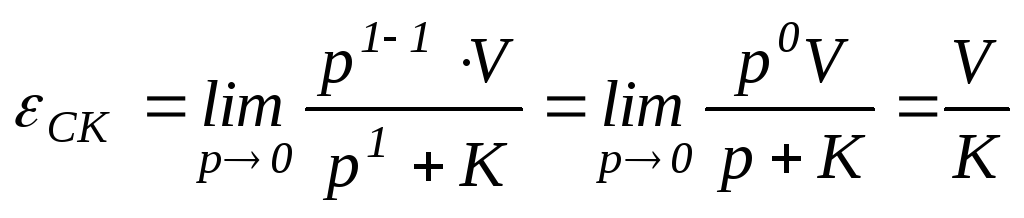
There is a speed error in a 1st order astatic self-propelled gun ε SK, which can only be reduced by increasing the overall gain TO open ACS, but it cannot be turned to zero.

3). Let in (1.58) the value of the order ν astatism of self-propelled guns is 2: ν=2. Such an automatic control system is called astatic 2nd order. Then speed error ε SK will be equal

In a 2nd order astatic self-propelled gun, speed error ε SK equal to zero, i.e. the ACS is absolutely accurate.

Conclusions from the calculations of static and speed control errors:

1. Control errors can be reduced by increasing the overall gain TO and the order of astatism ν open ACS.

2. When increasing TO control errors are only decreasing. but do not go to zero.

3. When increasing ν The ACS becomes absolutely accurate - the control error becomes zero.

Indirect quality indicators of automatic control systems and their relationship with direct quality indicators. Using LFC to assess the quality of self-propelled guns

The impossibility of obtaining formulas for calculating dynamic quality indicators (Fig. 1.42), as well as the requirements of the tasks of ACS synthesis, led to the development of complex quality indicators. Indirect quality indicators, for the most part, are frequency, which are determined from the frequency response, frequency response, phase response and LFC. Indirect quality indicators must meet the following requirements:

1. Indirect indicators should simply be calculated or determined from the frequency characteristics of an open-loop automatic control system.

2. The error in determining the values ​​of direct quality indicators through the values ​​of indirect quality indicators should be small.

3. Indirect indicators must be adapted to effectively solve problems of ACS synthesis.

4
. Indirect indicators should make it possible to simply analyze the influence of the settings of the ACS regulators and the characteristics of any other parts of the ACS on direct quality indicators.

Quite a lot of indirect quality indicators or sets of them have been developed. Each indirect quality indicator or a set of them is introduced to effectively solve specific types of automatic control problems and, therefore, universal indirect quality indicators do not exist in principle. In fact, indirect indicators simplify the analysis and synthesis of automatic control systems, but direct quality indicators are always determined inaccurately through indirect indicators.

First of all, consider a set of indirect quality indicators obtained from Nyquist constructions (see topic 1.12): cutoff frequency ω SR and phase margin γ . Cutoff frequency ω SR simply determined from the LFC (Fig. 1.41). Phase margin γ calculated by the expression FCHH φ (ω ) only at one frequency value ω SR :γ=φ (ω SR ).

The basis for the use of indirect quality indicators is the cutoff frequency ω SR and phase reserve γ - there are graphical dependencies (Fig. 14.1) between indirect and direct quality indicators - overshoot σ , time of first installation t 1 and the time of the transition process t PP .

The ordinate axis shows the overshoot values σ , as a percentage of the steady value h ycm(Fig. 1.42). Along the axis of time t 1 And t PP written down formulas that are used to calculate t 1 And t PP depending on cutoff frequency ω SR. If the phase margin values ​​are determined from the frequency characteristics γ and cutoff frequencies ω SR, then from the graphs you can determine the overshoot values σ , time of first installation t 1 and transition time t PP. For example, let the values ​​be given γ=30 O And ω SR =1.5 s -1 . Then, according to the constructions shown in Fig. 1.44, we obtain:

σ=19%,

Found values σ, t 1 And t PP are not accurate. This fact is reflected in Fig. 1.44 as the “blurring” of the graphs.

According to these values σ ,t 1 And t PP you can build an approximate graph of the transition process (Fig. 1.45). As is customary, indirect quality indicators are chosen such that the estimates of direct quality indicators found with their help would have an error of no more than 10%. This is quite acceptable in engineering practice.

Graphical dependencies between indirect γ And ω SR and straight σ ,t 1 And t PP The quality indicators of the ACS shown in Fig. 1.44 can be described in the form of the following proportional type dependencies

The task of determining the influence of standard control laws (proportional, integral and differential) on direct quality indicators, which is important in the practice of operating automatic control systems, is extremely effectively solved using the introduced indirect indicators γ And ω SR .

H
The frequency method for synthesizing a tracking automatic control system (see topic 1.23) is based on the use of an indirect quality indicator - the oscillation indicator M. Visibility indicator M is a value that is numerically equal to the maximum of the normalized frequency response (Fig. 1.46). According to the value of the oscillation index M it is possible to estimate the amount of overshoot σ (Fig. 1.47).

The value of the oscillation index M can be found graphically, without calculating the frequency response, using only the frequency response hodograph W once (p) and, accordingly, the LFC of the open ACS. It is these constructions that form the basis for calculating the mid-frequency section of the desired LFC during the above-mentioned frequency synthesis of the tracking ACS.

Requirements

ACS steering device.

the drive must provide shifting from -35˚ to +30˚ in 28s.

At in full swing within 1 hour the drive must provide 350 transfers.

Control stations must be equipped with axiometers with an accuracy of 1º in DP and 1.5º at α = ± 5º. At large angles±2.5º

Requirements for SEES:

A) static requirements:

Frequency regulation error - less than 5%

Voltage regulation error - -10 to +6%

Uneven load distribution of parallel operating generators: no more than 10% of the power of the largest generator or no more than 25% of the power of the smallest generator. Of the two options, or choose the smaller one.

B) dynamic indicators

Frequency overshoot/failure – no more than 10% for 5 seconds

Voltage surge/dip – no more than 20% for 1.5 seconds

Requirements of DAU GD

The frequency regulator must be all-mode, permissible frequency adjustment ranges from 40 to 115%

There should be no time delay between moving the handle on the bridge and the beginning of the rotation of the blades and the diesel engine speed

Frequency maintenance accuracy is no worse than 1.5%

Several control posts for the main engine and propeller must be implemented, namely from different positions, during acceleration and release, during reverse, when controlling the main engine when it is included in the ship’s network

The start of the reversing characteristics of the main engine must be commensurate with qualified manual control

List typical positional, integrating and differentiating elements of self-propelled control systems and give examples of them from ship automation systems. Specify the transfer functions and transient characteristics

these links.

Types of typical positional links: 1. Inertia-free (proportional) link W(p)= has a transfer function and is described by an algebraic equation, respectively, of the form, k= y

kx

Examples of inertia-free links are a lever transmission (Fig. 1.10a), a potentiometric displacement sensor (Fig. 1.10b). In these links the output signal at repeats the input signal without delay.

X k= y

Transient Expression 2. Aperiodic (inertial) link of the 1st order

has a transfer function and is described by an equation of the form has a transfer function and is described by an algebraic equation, respectively, of the formWhere, T -

transmission coefficient and link time constant. Examples of this link are the integrating- R.C.

circuit (Fig. 1.11a), “an electric motor, the windings of which heat up during operation (Fig. 1.11b). Examples of this link are the integrating- Let us derive the transfer function for

chains. Using Ohm's law, we get

The transient process is described by the expression x=1(t) where instead , as it should be for the transient process, is accepted actual value x signal

, due to which the reaction of the link to a jump of arbitrary magnitude is calculated. k The transition process graph is shown in Fig. 1.11c. Steady value mouth y, equal t . , is achieved at infinity: t Transition time , pp In these links the output signal The transition process graph is shown in Fig. 1.11c. Steady value determined by the moment the schedule finally enters the 5% tolerance zone from 3 , is. T The link has self-leveling

3
. The property of self-leveling is that the link independently, without the use of additional regulation, comes to a steady value that is constant in magnitude.. Inertial link of the 2nd order

has a transfer function

The peculiarity of the link is that its characteristic equation has real roots. Examples of this link are RLC - circuit (Fig. 1.13a) with high resistance R
resistor , an electric drive that rotates a load with a large moment of inertia J

(Fig. 6.4b).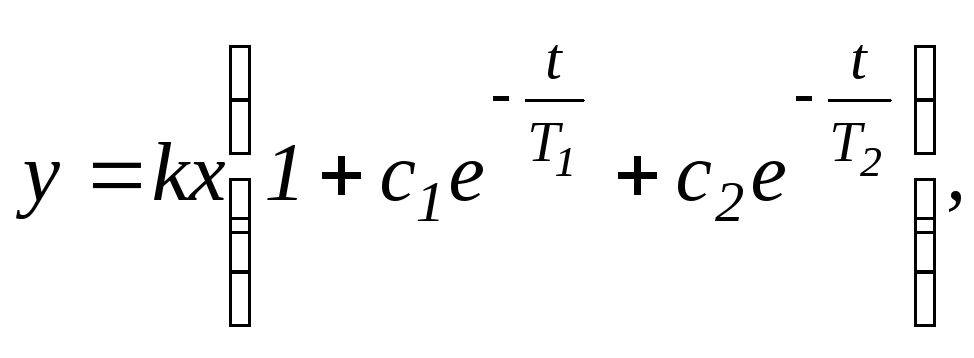

has a transfer function and is described by an equation of the form The transient process is described by the expression 1 And With 2 With

- constant integrations.
G t Transition time The transition process graph (Fig. 1.14a) has an inflection point. Transition time

can only be determined graphically.. Inertial link of the 2nd order

has a transfer function and is described by an equation of the form , is- period of free (undamped) oscillations;

ξ - attenuation parameter taking values 0< ξ <1.

The peculiarity of the link is that its characteristic equation has complex conjugate roots.

The peculiarity of the link is that its characteristic equation has real roots. Examples of this link are- circuit (Fig. 1.13a) with low resistance - circuit (Fig. 1.13a) with high resistance R
, an electric drive that rotates a load with a low moment of inertia , an electric drive that rotates a load with a large moment of inertia(Fig. 1.13b). The transient process is described by the expression

has a transfer function and is described by an equation of the form
- resonant frequency taking into account the damping of oscillations.

The transition process graph is shown in Fig. 1.14b. The lower the parameter value ξ , the slower the transient process decays. The transient time can only be determined graphically.