Sample confidence interval. Determining the confidence interval

Confidence interval

Confidence interval- a term used in mathematical statistics for interval (as opposed to point) estimation of statistical parameters, which is preferable when the sample size is small. A confidence interval is one that covers an unknown parameter with a given reliability.

The method of confidence intervals was developed by the American statistician Jerzy Neumann, based on the ideas of the English statistician Ronald Fisher.

Definition

Confidence interval of the parameter θ random variable distribution X with confidence level 100 p%, generated by the sample ( x 1 ,…,x n), is called an interval with boundaries ( x 1 ,…,x n) and ( x 1 ,…,x n), which are realizations of random variables L(X 1 ,…,X n) and U(X 1 ,…,X n), such that

The boundary points of the confidence interval are called confidence limits.

An intuition-based interpretation of the confidence interval would be: if p is large (say 0.95 or 0.99), then the confidence interval almost certainly contains the true value θ .

Another interpretation of the concept of a confidence interval: it can be considered as an interval of parameter values θ compatible with experimental data and not contradicting them.

Examples

Confidence interval for the mathematical expectation of a normal sample;
Confidence interval for normal sample variance.

Bayesian confidence interval

In Bayesian statistics, there is a similar but different in some key details definition of a confidence interval. Here, the estimated parameter itself is considered a random variable with some given prior distribution (in the simplest case, uniform), and the sample is fixed (in classical statistics everything is exactly the opposite). A Bayesian confidence interval is an interval covering the parameter value with the posterior probability:

In general, classical and Bayesian confidence intervals are different. In the English-language literature, the Bayesian confidence interval is usually called the term credible interval, and the classic one - confidence interval.

Notes

Sources

Wikimedia Foundation.

2010.
Kids (film)

Colonist

Confidence interval- an interval calculated from sample data, which with a given probability (confidence) covers the unknown true value of the estimated distribution parameter. Source: GOST 20522 96: Soils. Methods for statistical processing of results... Dictionary-reference book of terms of normative and technical documentation

confidence interval- for a scalar parameter of the population, this is a segment that most likely contains this parameter. This phrase is meaningless without further elaboration. Since the boundaries of the confidence interval are estimated from the sample, it is natural to... ... Dictionary of Sociological Statistics

CONFIDENCE INTERVAL- a method of estimating parameters that differs from point estimation. Let the sample x1, . . ., xn from a distribution with probability density f(x, α), and a*=a*(x1, . . ., xn) estimate α, g(a*, α) probability density estimate. Are looking for… … Geological encyclopedia

CONFIDENCE INTERVAL- (confidence interval) An interval in which the reliability of the parameter value for the population obtained on the basis of a sample survey has a certain degree of probability, for example 95%, which is due to the sample itself. Width… … Economic dictionary

confidence interval- is the interval in which the true value of the determined quantity is located with a given confidence probability. General chemistry: textbook / A. V. Zholnin ... Chemical terms

Confidence interval CI- Confidence interval, CI * data interval, CI * confidence interval interval of the characteristic value, calculated for k.l. distribution parameter (for example, the average value of a characteristic) across the sample and with a certain probability (for example, 95% for 95% ... Genetics. encyclopedic Dictionary

CONFIDENCE INTERVAL- a concept that arises when estimating a statistical parameter. distribution by interval of values. D. and. for parameter q, corresponding to this coefficient. trust P is equal to such an interval (q1, q2) that for any probability distribution of inequality... ... Physical encyclopedia

confidence interval- - Telecommunications topics, basic concepts EN confidence interval ... Technical Translator's Guide

confidence interval- pasikliovimo intervalas statusas T sritis Standartizacija ir metrologija apibrėžtis Dydžio verčių intervalas, kuriame su pasirinktąja tikimybe yra matavimo rezultato vertė. atitikmenys: engl. confidence interval vok. Vertrauensbereich, m rus.… … Penkiakalbis aiškinamasis metrologijos terminų žodynas

confidence interval- pasikliovimo intervalas statusas T sritis chemija apibrėžtis Dydžio verčių intervalas, kuriame su pasirinktąja tikimybe yra matavimo rezultatų vertė. atitikmenys: engl. confidence interval rus. trust area; confidence interval... Chemijos terminų aiškinamasis žodynas

Target– teach students algorithms for calculating confidence intervals of statistical parameters.

When statistically processing data, the calculated arithmetic mean, coefficient of variation, correlation coefficient, difference criteria and other point statistics should receive quantitative confidence limits, which indicate possible fluctuations of the indicator in smaller and larger directions within the confidence interval.

Example 3.1 . The distribution of calcium in the blood serum of monkeys, as previously established, is characterized by the following sample indicators: = 11.94 mg%; = 0.127 mg%; n= 100. It is required to determine the confidence interval for the general average ( ) with confidence probability P = 0,95.

The general average is located with a certain probability in the interval:

, Where – sample arithmetic mean; t– Student’s test; – arithmetic mean error.

Using the table “Student’s t-test values” we find the value with a confidence probability of 0.95 and the number of degrees of freedom k= 100-1 = 99. It is equal to 1.982. Together with the values of the arithmetic mean and statistical error, we substitute it into the formula:

or 11.69
12,19

Thus, with a probability of 95%, it can be stated that the general average of this normal distribution is between 11.69 and 12.19 mg%.

Example 3.2 . Determine the boundaries of the 95% confidence interval for the general variance ( ) distribution of calcium in the blood of monkeys, if it is known that
= 1.60, at n = 100.

To solve the problem you can use the following formula:

Where – statistical error of dispersion.

We find the sampling variance error using the formula:
. It is equal to 0.11. Meaning t- criterion with a confidence probability of 0.95 and the number of degrees of freedom k= 100–1 = 99 is known from the previous example.

Let's use the formula and get:

or 1.38
1,82

More accurately, the confidence interval of the general variance can be constructed using (chi-square) - Pearson test. The critical points for this criterion are given in a special table. When using the criterion To construct a confidence interval, a two-sided significance level is used. For the lower limit, the significance level is calculated using the formula
, for the top –
. For example, for the confidence level = 0,99= 0,010,= 0.990. Accordingly, according to the table of distribution of critical values , with calculated confidence levels and number of degrees of freedom k= 100 – 1= 99, find the values
And
. We get
equals 135.80, and
equals 70.06.

To find confidence limits for the general variance using Let's use the formulas: for the lower boundary
, for the upper bound
. Let's substitute the found values for the problem data into formulas:
= 1,17;
= 2.26. Thus, with a confidence probability P= 0.99 or 99% general variance will lie in the range from 1.17 to 2.26 mg% inclusive.

Example 3.3 . Among 1000 wheat seeds from the batch received at the elevator, 120 seeds were found infected with ergot. It is necessary to determine the probable boundaries of the general proportion of infected seeds in a given batch of wheat.

It is advisable to determine the confidence limits for the general share for all its possible values using the formula:

Where n – number of observations; m– absolute size of one of the groups; t– normalized deviation.

The sample proportion of infected seeds is
or 12%. With confidence probability R= 95% normalized deviation ( t-Student's test at k =
)t = 1,960.

We substitute the available data into the formula:

Hence the boundaries of the confidence interval are equal to = 0.122–0.041 = 0.081, or 8.1%; = 0.122 + 0.041 = 0.163, or 16.3%.

Thus, with a confidence probability of 95% it can be stated that the general proportion of infected seeds is between 8.1 and 16.3%.

Example 3.4 . The coefficient of variation characterizing the variation of calcium (mg%) in the blood serum of monkeys was equal to 10.6%. Sample size n= 100. It is necessary to determine the boundaries of the 95% confidence interval for the general parameter Cv.

Limits of the confidence interval for the general coefficient of variation Cv are determined by the following formulas:

And
, Where K intermediate value calculated by the formula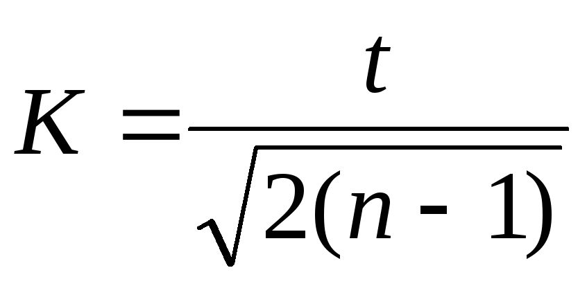
.

Knowing that with confidence probability R= 95% normalized deviation (Student's test at k =
)t = 1.960, let’s first calculate the value TO:

or 9.3%

or 12.3%

Thus, the general coefficient of variation with a 95% confidence level lies in the range from 9.3 to 12.3%. With repeated samples, the coefficient of variation will not exceed 12.3% and will not be below 9.3% in 95 cases out of 100.

Questions for self-control:

Problems for independent solution.

1. The average percentage of fat in milk during lactation of Kholmogory crossbred cows was as follows: 3.4; 3.6; 3.2; 3.1; 2.9; 3.7; 3.2; 3.6; 4.0; 3.4; 4.1; 3.8; 3.4; 4.0; 3.3; 3.7; 3.5; 3.6; 3.4; 3.8. Establish confidence intervals for the general mean at 95% confidence level (20 points).

2. On 400 hybrid rye plants, the first flowers appeared on average 70.5 days after sowing. The standard deviation was 6.9 days. Determine the error of the mean and confidence intervals for the general mean and variance at the significance level W= 0.05 and W= 0.01 (25 points).

3. When studying the length of leaves of 502 specimens of garden strawberries, the following data were obtained: = 7.86 cm; σ = 1.32 cm, =± 0.06 cm. Determine confidence intervals for the arithmetic population mean with significance levels of 0.01; 0.02; 0.05. (25 points).

4. In a study of 150 adult men, the average height was 167 cm, and σ = 6 cm. What are the limits of the general mean and general variance with a confidence probability of 0.99 and 0.95? (25 points).

5. The distribution of calcium in the blood serum of monkeys is characterized by the following selective indicators: = 11.94 mg%, σ = 1,27, n = 100. Construct a 95% confidence interval for the general mean of this distribution. Calculate the coefficient of variation (25 points).

6. The total nitrogen content in the blood plasma of albino rats at the age of 37 and 180 days was studied. The results are expressed in grams per 100 cm 3 of plasma. At the age of 37 days, 9 rats had: 0.98; 0.83; 0.99; 0.86; 0.90; 0.81; 0.94; 0.92; 0.87. At the age of 180 days, 8 rats had: 1.20; 1.18; 1.33; 1.21; 1.20; 1.07; 1.13; 1.12. Set confidence intervals for the difference at a confidence level of 0.95 (50 points).

7. Determine the boundaries of the 95% confidence interval for the general variance of the distribution of calcium (mg%) in the blood serum of monkeys, if for this distribution the sample size is n = 100, statistical error of the sample variance s σ 2 = 1.60 (40 points).

8. Determine the boundaries of the 95% confidence interval for the general variance of the distribution of 40 wheat spikelets along the length (σ 2 = 40.87 mm 2). (25 points).

9. Smoking is considered the main factor predisposing to obstructive pulmonary diseases. Passive smoking is not considered such a factor. Scientists doubted the harmlessness of passive smoking and examined the airway patency of non-smokers, passive and active smokers. To characterize the state of the respiratory tract, we took one of the indicators of external respiration function - the maximum volumetric flow rate of mid-expiration. A decrease in this indicator is a sign of airway obstruction. The survey data are shown in the table.

	Number of people examined	Maximum mid-expiratory flow rate, l/s
	Number of people examined		Standard deviation
Non-smokers
work in a non-smoking area
working in a smoky room
Smoking
smoke a small number of cigarettes
average number of cigarette smokers
smoke a large number of cigarettes

Using the table data, find 95% confidence intervals for the overall mean and overall variance for each group. What are the differences between the groups? Present the results graphically (25 points).

10. Determine the boundaries of the 95% and 99% confidence intervals for the general variance in the number of piglets in 64 farrows, if the statistical error of the sample variance s σ 2 = 8.25 (30 points).

11. It is known that the average weight of rabbits is 2.1 kg. Determine the boundaries of the 95% and 99% confidence intervals for the general mean and variance at n= 30, σ = 0.56 kg (25 points).

12. The grain content of the ear was measured for 100 ears ( X), ear length ( Y) and the mass of grain in the ear ( Z). Find confidence intervals for the general mean and variance at P 1 = 0,95, P 2 = 0,99, P 3 = 0.999 if = 19, = 6.766 cm, = 0.554 g; σ x 2 = 29.153, σ y 2 = 2. 111, σ z 2 = 0. 064. (25 points).

13. In 100 randomly selected ears of winter wheat, the number of spikelets was counted. The sample population was characterized by the following indicators: = 15 spikelets and σ = 2.28 pcs. Determine with what accuracy the average result was obtained ( ) and construct a confidence interval for the general mean and variance at 95% and 99% significance levels (30 points).

14. Number of ribs on fossil mollusk shells Orthambonites calligramma:

It is known that n = 19, σ = 4.25. Determine the boundaries of the confidence interval for the general mean and general variance at the significance level W = 0.01 (25 points).

15. To determine milk yield on a commercial dairy farm, the productivity of 15 cows was determined daily. According to data for the year, each cow gave on average the following amount of milk per day (l): 22; 19; 25; 20; 27; 17; thirty; 21; 18; 24; 26; 23; 25; 20; 24. Construct confidence intervals for the general variance and the arithmetic mean. Can we expect the average annual milk yield per cow to be 10,000 liters? (50 points).

16. In order to determine the average wheat yield for the agricultural enterprise, mowing was carried out on trial plots of 1, 3, 2, 5, 2, 6, 1, 3, 2, 11 and 2 hectares. Productivity (c/ha) from the plots was 39.4; 38; 35.8; 40; 35; 42.7; 39.3; 41.6; 33; 42; 29 respectively. Construct confidence intervals for the general variance and arithmetic mean. Can we expect that the average agricultural yield will be 42 c/ha? (50 points).

Confidence interval for mathematical expectation - this is an interval calculated from data that, with a known probability, contains the mathematical expectation of the general population. A natural estimate for the mathematical expectation is the arithmetic mean of its observed values. Therefore, throughout the lesson we will use the terms “average” and “average value”. In problems of calculating a confidence interval, an answer most often required is something like “The confidence interval of the mean [value in a particular problem] is from [smaller value] to [larger value].” Using a confidence interval, you can evaluate not only average values, but also the proportion of a particular characteristic of the general population. Average values, dispersion, standard deviation and error, through which we will arrive at new definitions and formulas, are discussed in the lesson Characteristics of the sample and population .

Point and interval estimates of the mean

If the average value of the population is estimated by a number (point), then a specific average, which is calculated from a sample of observations, is taken as an estimate of the unknown average value of the population. In this case, the value of the sample mean - a random variable - does not coincide with the mean value of the general population. Therefore, when indicating the sample mean, you must simultaneously indicate the sampling error. The measure of sampling error is the standard error, which is expressed in the same units as the mean. Therefore, the following notation is often used: .

If the estimate of the average needs to be associated with a certain probability, then the parameter of interest in the population must be estimated not by one number, but by an interval. A confidence interval is an interval in which, with a certain probability P the value of the estimated population indicator is found. Confidence interval in which it is probable P = 1 - α the random variable is found, calculated as follows:

α = 1 - P, which can be found in the appendix to almost any book on statistics.

In practice, the population mean and variance are not known, so the population variance is replaced by the sample variance, and the population mean by the sample mean. Thus, the confidence interval in most cases is calculated as follows:

The confidence interval formula can be used to estimate the population mean if

the standard deviation of the population is known;
or the standard deviation of the population is unknown, but the sample size is greater than 30.

The sample mean is an unbiased estimate of the population mean. In turn, the sample variance is not an unbiased estimate of the population variance. To obtain an unbiased estimate of the population variance in the sample variance formula, sample size n should be replaced by n-1.

Example 1. Information was collected from 100 randomly selected cafes in a certain city that the average number of employees in them is 10.5 with a standard deviation of 4.6. Determine the 95% confidence interval for the number of cafe employees.

where is the critical value of the standard normal distribution for the significance level α = 0,05 .

Thus, the 95% confidence interval for the average number of cafe employees ranged from 9.6 to 11.4.

Example 2. For a random sample from a population of 64 observations, the following total values were calculated:

sum of values in observations,

sum of squared deviations of values from the mean .

Calculate the 95% confidence interval for the mathematical expectation.

Let's calculate the standard deviation:

Let's calculate the average value:

We substitute the values into the expression for the confidence interval:

where is the critical value of the standard normal distribution for the significance level α = 0,05 .

We get:

Thus, the 95% confidence interval for the mathematical expectation of this sample ranged from 7.484 to 11.266.

Example 3. For a random population sample of 100 observations, the calculated mean is 15.2 and standard deviation is 3.2. Calculate the 95% confidence interval for the expected value, then the 99% confidence interval. If the sample power and its variation remain unchanged and the confidence coefficient increases, will the confidence interval narrow or widen?

We substitute these values into the expression for the confidence interval:

where is the critical value of the standard normal distribution for the significance level α = 0,05 .

We get:

Thus, the 95% confidence interval for the mean of this sample ranged from 14.57 to 15.82.

We again substitute these values into the expression for the confidence interval:

where is the critical value of the standard normal distribution for the significance level α = 0,01 .

We get:

Thus, the 99% confidence interval for the mean of this sample ranged from 14.37 to 16.02.

As we see, as the confidence coefficient increases, the critical value of the standard normal distribution also increases, and, consequently, the starting and ending points of the interval are located further from the mean, and thus the confidence interval for the mathematical expectation increases.

Point and interval estimates of specific gravity

The share of some sample attribute can be interpreted as a point estimate of the share p the same characteristic in the general population. If this value needs to be associated with probability, then the confidence interval of the specific gravity should be calculated p characteristic in the population with probability P = 1 - α :

Example 4. In some city there are two candidates A And B are running for mayor. 200 city residents were randomly surveyed, of which 46% responded that they would vote for the candidate A, 26% - for the candidate B and 28% do not know who they will vote for. Determine the 95% confidence interval for the proportion of city residents supporting the candidate A.

Confidence interval– the limiting values of a statistical quantity that, with a given confidence probability γ, will be in this interval when sampling a larger volume. Denoted as P(θ - ε. In practice, the confidence probability γ is chosen from values quite close to unity: γ = 0.9, γ = 0.95, γ = 0.99.

Purpose of the service. Using this service, you can determine:

confidence interval for the general mean, confidence interval for the variance;
confidence interval for the standard deviation, confidence interval for the general share;

The resulting solution is saved in a Word file (see example). Below is a video instruction on how to fill out the initial data.

Example No. 1. On a collective farm, out of a total herd of 1000 sheep, 100 sheep underwent selective control shearing. As a result, an average wool clipping of 4.2 kg per sheep was established. Determine with a probability of 0.99 the mean square error of the sample when determining the average wool shearing per sheep and the limits within which the shearing value is contained if the variance is 2.5. The sample is non-repetitive.
Example No. 2. From a batch of imported products at the post of the Moscow Northern Customs, 20 samples of product “A” were taken by random repeated sampling. As a result of the test, the average moisture content of product “A” in the sample was established, which turned out to be equal to 6% with a standard deviation of 1%.
Determine with probability 0.683 the limits of the average moisture content of the product in the entire batch of imported products.
Example No. 3. A survey of 36 students showed that the average number of textbooks read by them during the academic year was equal to 6. Assuming that the number of textbooks read by a student per semester has a normal distribution law with a standard deviation equal to 6, find: A) with a reliability of 0 .99 interval estimate for the mathematical expectation of this random variable; B) with what probability can we say that the average number of textbooks read by a student per semester, calculated from this sample, will deviate from the mathematical expectation in absolute value by no more than 2.

Classification of confidence intervals

By type of parameter being assessed:

By sample type:

Confidence interval for an infinite sample;
Confidence interval for the final sample;

The sample is called resampling, if the selected object is returned to the population before selecting the next one. The sample is called non-repeat, if the selected object is not returned to the population. In practice, we usually deal with non-repetitive samples.

Calculation of the average sampling error for random sampling

The discrepancy between the values of indicators obtained from the sample and the corresponding parameters of the general population is called representativeness error.
Designations of the main parameters of the general and sample populations.

Average sampling error formulas
re-selection		non-repetitive selection
for average	for share	for average	for share

The relationship between the sampling error limit (Δ) guaranteed with some probability Р(t), and the average sampling error has the form: or Δ = t·μ, where t– confidence coefficient, determined depending on the probability level P(t) according to the table of Laplace integral function.

Formulas for calculating the sample size using a purely random sampling method

In the previous subsections we considered the issue of estimating an unknown parameter A one number. This is called a “point” estimate. In a number of tasks, you not only need to find for the parameter A suitable numerical value, but also to evaluate its accuracy and reliability. You need to know what errors replacing a parameter can lead to A its point estimate A and with what degree of confidence can we expect that these errors will not exceed known limits?

Problems of this kind are especially relevant with a small number of observations, when the point estimate and in is largely random and approximate replacement of a by a can lead to serious errors.

To give an idea of the accuracy and reliability of the estimate A,

In mathematical statistics, so-called confidence intervals and confidence probabilities are used.

Let for the parameter A unbiased estimate obtained from experience A. We want to estimate the possible error in this case. Let us assign some sufficiently large probability p (for example, p = 0.9, 0.95 or 0.99) such that an event with probability p can be considered practically reliable, and find a value s for which

Then the range of practically possible values of the error arising during replacement A on A, will be ± s; Large errors in absolute value will appear only with a low probability a = 1 - p. Let's rewrite (14.3.1) as:

Equality (14.3.2) means that with probability p the unknown value of the parameter A falls within the interval

It is necessary to note one circumstance. Previously, we have repeatedly considered the probability of a random variable falling into a given non-random interval. Here the situation is different: the magnitude A is not random, but the interval / p is random. Its position on the x-axis is random, determined by its center A; In general, the length of the interval 2s is also random, since the value of s is calculated, as a rule, from experimental data. Therefore, in this case, it would be better to interpret the p value not as the probability of “hitting” the point A in the interval / p, and as the probability that a random interval / p will cover the point A(Fig. 14.3.1).

Rice. 14.3.1

The probability p is usually called confidence probability, and interval / p - confidence interval. Interval boundaries If. a x = a- s and a 2 = a + and are called trust boundaries.

Let's give another interpretation to the concept of a confidence interval: it can be considered as an interval of parameter values A, compatible with experimental data and not contradicting them. Indeed, if we agree to consider an event with probability a = 1-p practically impossible, then those values of the parameter a for which a - a> s must be recognized as contradicting experimental data, and those for which |a - A a t na 2 .

Let for the parameter A there is an unbiased estimate A. If we knew the law of distribution of the quantity A, the task of finding a confidence interval would be very simple: it would be enough to find a value s for which

The difficulty is that the law of distribution of estimates A depends on the distribution law of the quantity X and, therefore, on its unknown parameters (in particular, on the parameter itself A).

To get around this difficulty, you can use the following roughly approximate technique: replace the unknown parameters in the expression for s with their point estimates. With a relatively large number of experiments P(about 20...30) this technique usually gives results that are satisfactory in terms of accuracy.

As an example, consider the problem of a confidence interval for the mathematical expectation.

Let it be produced P X, whose characteristics are the mathematical expectation T and variance D- unknown. The following estimates were obtained for these parameters:

It is required to construct a confidence interval / p corresponding to the confidence probability p for the mathematical expectation T quantities X.

When solving this problem, we will use the fact that the quantity T represents the sum P independent identically distributed random variables Xh and according to the central limit theorem, for a sufficiently large P its distribution law is close to normal. In practice, even with a relatively small number of terms (about 10...20), the distribution law of the sum can be approximately considered normal. We will assume that the value T distributed according to the normal law. The characteristics of this law - mathematical expectation and variance - are equal, respectively T And

(see chapter 13 subsection 13.3). Let us assume that the value D we know and will find a value Ep for which

Using formula (6.3.5) of Chapter 6, we express the probability on the left side of (14.3.5) through the normal distribution function

where is the standard deviation of the estimate T.

From Eq.

find the value of Sp:

where arg Ф* (х) is the inverse function of Ф* (X), those. such a value of the argument for which the normal distribution function is equal to X.

Dispersion D, through which the quantity is expressed A 1P, we do not know exactly; as its approximate value, you can use the estimate D(14.3.4) and put approximately:

Thus, the problem of constructing a confidence interval has been approximately solved, which is equal to:

where gp is determined by formula (14.3.7).

To avoid reverse interpolation in the tables of the function Ф* (l) when calculating s p, it is convenient to compile a special table (Table 14.3.1), which gives the values of the quantity

depending on r. The value (p determines for the normal law the number of standard deviations that must be plotted to the right and left from the center of dispersion so that the probability of getting into the resulting area is equal to p.

Using the value 7 p, the confidence interval is expressed as:

Table 14.3.1

Example 1. 20 experiments were carried out on the quantity X; the results are shown in table. 14.3.2.

Table 14.3.2

It is required to find an estimate from for the mathematical expectation of the quantity X and construct a confidence interval corresponding to the confidence probability p = 0.8.

Solution. We have:

Choosing l: = 10 as the reference point, using the third formula (14.2.14) we find the unbiased estimate D :

According to the table 14.3.1 we find

Confidence limits:

Confidence interval:

Parameter values T, lying in this interval are compatible with the experimental data given in table. 14.3.2.

A confidence interval for the variance can be constructed in a similar way.

Let it be produced P independent experiments on a random variable X with unknown parameters for both A and dispersion D an unbiased estimate was obtained:

It is required to approximately construct a confidence interval for the variance.

From formula (14.3.11) it is clear that the quantity D represents

amount P random variables of the form . These values are not

independent, since any of them includes the quantity T, dependent on everyone else. However, it can be shown that with increasing P the law of distribution of their sum also approaches normal. Almost at P= 20...30 it can already be considered normal.

Let's assume that this is so and find the characteristics of this law: mathematical expectation and dispersion. Since the assessment D- unbiased, then M[D] = D.

Variance calculation D D is associated with relatively complex calculations, so we present its expression without derivation:

where q 4 is the fourth central moment of the magnitude X.

To use this expression, you need to substitute the values \u003d 4 and D(at least close ones). Instead of D you can use his assessment D. In principle, the fourth central moment can also be replaced by an estimate, for example, a value of the form:

but such a replacement will give extremely low accuracy, since in general, with a limited number of experiments, high-order moments are determined with large errors. However, in practice it often happens that the type of quantity distribution law X known in advance: only its parameters are unknown. Then you can try to express μ 4 through D.

Let's take the most common case, when the value X distributed according to the normal law. Then its fourth central moment is expressed in terms of dispersion (see Chapter 6, subsection 6.2);

and formula (14.3.12) gives or

Replacing the unknown in (14.3.14) D his assessment D, we get: from where

Moment μ 4 can be expressed through D also in some other cases, when the distribution of the value X is not normal, but its appearance is known. For example, for the law of uniform density (see Chapter 5) we have:

where (a, P) is the interval on which the law is specified.

Hence,

Using formula (14.3.12) we obtain: where do we find approximately

In cases where the type of the distribution law for the quantity 26 is unknown, when making an approximate estimate of the value a/) it is still recommended to use formula (14.3.16), unless there are special reasons to believe that this law is very different from the normal one (has a noticeable positive or negative kurtosis) .

If the approximate value a/) is obtained in one way or another, then we can construct a confidence interval for the variance in the same way as we built it for the mathematical expectation:

where the value depending on the given probability p is found according to the table. 14.3.1.

Example 2. Find approximately 80% confidence interval for the variance of a random variable X under the conditions of example 1, if it is known that the value X distributed according to a law close to normal.

Solution. The value remains the same as in the table. 14.3.1:

According to formula (14.3.16)

Using formula (14.3.18) we find the confidence interval:

The corresponding range of standard deviation values: (0.21; 0.29).

14.4. Exact methods for constructing confidence intervals for the parameters of a random variable distributed according to a normal law

In the previous subsection, we examined roughly approximate methods for constructing confidence intervals for mathematical expectation and variance. Here we will give an idea of the exact methods to solve the same problem. We emphasize that in order to accurately find confidence intervals it is absolutely necessary to know in advance the form of the distribution law of the quantity X, whereas for the application of approximate methods this is not necessary.

The idea of accurate methods for constructing confidence intervals comes down to the following. Any confidence interval is found from a condition expressing the probability of fulfilling certain inequalities, which include the estimate we are interested in A. Law of valuation distribution A in the general case depends on unknown parameters of the quantity X. However, sometimes it is possible to pass in inequalities from a random variable A to some other function of observed values X p X 2, ..., X p. the distribution law of which does not depend on unknown parameters, but depends only on the number of experiments and on the type of distribution law of the quantity X. These kinds of random variables play an important role in mathematical statistics; they have been studied in most detail for the case of a normal distribution of the quantity X.

For example, it has been proven that with a normal distribution of the value X random value

obeys the so-called Student distribution law With P- 1 degrees of freedom; the density of this law has the form

where G(x) is the known gamma function:

It has also been proven that the random variable

has a "distribution %2" with P- 1 degrees of freedom (see Chapter 7), the density of which is expressed by the formula

Without dwelling on the derivations of distributions (14.4.2) and (14.4.4), we will show how they can be applied when constructing confidence intervals for parameters ty D.

Let it be produced P independent experiments on a random variable X, normally distributed with unknown parameters T&O. For these parameters, estimates were obtained

It is required to construct confidence intervals for both parameters corresponding to the confidence probability p.

Let's first construct a confidence interval for the mathematical expectation. It is natural to take this interval symmetrical with respect to T; let s p denote half the length of the interval. The value s p must be chosen so that the condition is satisfied

Let's try to move on the left side of equality (14.4.5) from the random variable T to a random variable T, distributed according to Student's law. To do this, multiply both sides of the inequality |m-w?|

by a positive value: or, using notation (14.4.1),

Let us find a number /p such that the value /p can be found from the condition

From formula (14.4.2) it is clear that (1) is an even function, therefore (14.4.8) gives

Equality (14.4.9) determines the value / p depending on p. If you have at your disposal a table of integral values

then the value of /p can be found by reverse interpolation in the table. However, it is more convenient to draw up a table of /p values in advance. Such a table is given in the Appendix (Table 5). This table shows the values depending on the confidence level p and the number of degrees of freedom P- 1. Having determined / p from the table. 5 and assuming

we will find half the width of the confidence interval / p and the interval itself

Example 1. 5 independent experiments were performed on a random variable X, normally distributed with unknown parameters T and about. The results of the experiments are given in table. 14.4.1.

Table 14.4.1

Find rating T for the mathematical expectation and construct a 90% confidence interval / p for it (i.e., the interval corresponding to the confidence probability p = 0.9).

Solution. We have:

According to table 5 of the application for P - 1 = 4 and p = 0.9 we find where

The confidence interval will be

Example 2. For the conditions of example 1 of subsection 14.3, assuming the value X normally distributed, find the exact confidence interval.

Solution. According to table 5 of the appendix we find when P - 1 = 19ir =

0.8 / p = 1.328; from here

Comparing with the solution of example 1 of subsection 14.3 (e p = 0.072), we are convinced that the discrepancy is very insignificant. If we maintain the accuracy to the second decimal place, then the confidence intervals found by the exact and approximate methods coincide:

Let's move on to constructing a confidence interval for the variance. Consider the unbiased variance estimator

and express the random variable D through magnitude V(14.4.3), having distribution x 2 (14.4.4):

Knowing the law of distribution of quantity V, you can find the interval /(1) in which it falls with a given probability p.

Law of distribution kn_x(v) magnitude I 7 has the form shown in Fig. 14.4.1.

Rice. 14.4.1

The question arises: how to choose the interval / p? If the law of distribution of magnitude V was symmetric (like the normal law or the Student distribution), it would be natural to take the interval /p symmetric with respect to the mathematical expectation. In this case the law k p_x (v) asymmetrical. Let us agree to choose the interval /p so that the probability of the value being V beyond the interval to the right and left (shaded areas in Fig. 14.4.1) were the same and equal

To construct an interval /p with this property, we use the table. 4 applications: it contains numbers y) such that

for the value V, having x 2 -distribution with r degrees of freedom. In our case r = n- 1. Let's fix r = n- 1 and find in the corresponding row of the table. 4 two meanings x 2 - one corresponding to probability the other - probability Let us denote these

values at 2 And xl? The interval has y 2, with your left, and y ~ right end.

Now let us find from the interval / p the desired confidence interval /|, for the dispersion with boundaries D, and D2, which covers the point D with probability p:

Let us construct an interval / (, = (?> ь А) that covers the point D if and only if the value V falls into the interval /r. Let us show that the interval

satisfies this condition. Indeed, the inequalities are equivalent to inequalities

and these inequalities are satisfied with probability p. Thus, the confidence interval for the variance has been found and is expressed by formula (14.4.13).

Example 3. Find the confidence interval for the variance under the conditions of example 2 of subsection 14.3, if it is known that the value X normally distributed.

Solution. We have . According to table 4 of the appendix

we find at g = n - 1 = 19

Using formula (14.4.13) we find the confidence interval for the variance

The corresponding interval for the standard deviation is (0.21; 0.32). This interval only slightly exceeds the interval (0.21; 0.29) obtained in example 2 of subsection 14.3 using the approximate method.

Figure 14.3.1 considers a confidence interval symmetric about a. In general, as we will see later, this is not necessary.