Mean value theorem. If f(x) is continuous on the interval, then there exists a point such that  . Doc. A function continuous on an interval takes on its smallest m and largest M values on this segment. Then
  . Number
  is concluded between the minimum and maximum values of the function on the segment. One of the properties of a function that is continuous on an interval is that this function takes any value located between m and M. Thus, there is a point such that
  . This property has a simple geometric interpretation: if continuous on the segment , then there is a point such that the area of the curvilinear trapezoid ABCD is equal to the area of the rectangle with base and height f(c) (highlighted in the figure).
7. Integral with variable upper limit. Its continuity and differentiability.
Let us consider a function f (x) that is Riemann integrable on the interval . Since it is integrable on , then it is also integrable on ∀x ∈ . Then for each x ∈ the expression makes sense, and for each x it is equal to a certain number.
Thus, each x ∈ is associated with a certain number,
those. the function is given:
(3.1)
Definition:
The function F (x) defined in (3.1), as well as the expression itself, is called
integral with a variable upper limit. It is defined over the entire segment
integrability of the function f (x).
Condition: f (t) is continuous on , and the function F (x) is given by formula (3.1).
Statement: The function F(x) is differentiable on , and F (x) = f (x).
(At point a it is right differentiable, and at point b it is left differentiable.)
Proof:
Since for a function of one variable F (x) differentiability is equivalent to the existence of a derivative at all points (at point a on the right, and at point b on the left), we will find the derivative of F (x). Let's consider the difference
Thus,
in this case, the point ξ lies on the segment (or if ∆x< 0).
Now remember that the derivative of the function F(x) at a given point x ∈ is equal to the limit of the difference ratio: . From the equality we have:
![]() ,
,
Now directing ∆x → 0, on the left side of this equality we obtain F’(x), and on the right side
Let us recall the definition of continuity of the function f (t) at point x:
Let x1 in this definition be equal to ξ. Since ξ ∈ (ξ ∈ ), and
∆x → 0, then |x − ξ| → 0, and by the definition of continuity, f (ξ) → f (x). From here we have:
F’(x) = f (x).
Consequence:
Condition: f (x) is continuous on .
Statement: Any antiderivative of the function f (x) has the form
![]()
where C ∈ R is some constant.
Proof. By Theorem 3.1 the function is an antiderivative for f(x). Suppose that G(x) is another antiderivative of f (x). Then G’(x) = f(x) and for the function F(x) − G(x) we have: (F (x) + G(x))’ = F’(x)−G’(x) = f (x)−f(x) ≡ 0. Hence, the derivative of the function F (x)−G(x)
is equal to zero, therefore, this function is constant: F(x) − G(x) = const.
8. Newton-Leibniz formula for a definite integral.
Theorem:
Condition: f(t) is continuous on , and F(x) is any antiderivative of it.
Statement:
Proof: Consider some antiderivative F (x) of the function f (x). According to the Corollary from the Theorem “On the differentiability of an integral with a variable upper limit” (see the previous question), it has the form . From here
 =>
c=
F(a)
, And
=>
c=
F(a)
, And
Let us move F(a) in the last equality to the left side, redesignate the integration variable again as x and obtain the Newton–Leibniz formula:
![]()
Theorem. If the function f(x) integrable on the interval [ a, b], Where a< b , and for everyone x ∈ inequality holds

Using the inequalities from the theorem, one can estimate the definite integral, i.e. indicate the boundaries between which its meaning is contained. These inequalities express an estimate of the definite integral.
Theorem [Mean Theorem]. If the function f(x) integrable on the interval [ a, b] and for everyone x ∈ the inequalities are satisfied m ≤ f(x) ≤ M, That

Where m ≤ μ ≤ M.
Comment. In case the function f(x) is continuous on the interval [ a, b], the equality from the theorem takes the form

Where c ∈. Number μ=f(c), defined by this formula, is called average value functions f(x) on the segment [ a, b]. This equality has the following geometric meaning: area of a curved trapezoid bounded by a continuous line y=f(x) (f(x) ≤ 0), is equal to the area of a rectangle with the same base and height equal to the ordinate of some point on this line.
Existence of an antiderivative for a continuous function
First, we introduce the concept of an integral with a variable upper limit.
Let the function f(x) integrable on the interval [ a, b]. Then whatever the number is x from [ a, b], function f(x) integrable on the interval [ a, b]. Therefore, on the interval [ a, b] function defined

which is called an integral with a variable upper limit.
Theorem. If the integrand is continuous on the interval [ a, b], then the derivative of a definite integral with a variable upper limit exists and is equal to the value of the integrand for this limit, that is
![]()
Consequence. A definite integral with a variable upper limit is one of the antiderivatives for a continuous integrand. In other words, for any function continuous on an interval there is an antiderivative.
Note 1. Note that if the function f(x) integrable on the interval [ a, b], then the integral with a variable upper limit is a function of the upper limit, continuous on this segment. Indeed, from St.2 and the mean value theorem we have
Note 2. The integral with a variable upper limit of integration is used in the definition of many new functions, for example, ![]() . These functions are not basic; as already noted, the antiderivatives of the indicated integrands are not expressed through elementary functions.
. These functions are not basic; as already noted, the antiderivatives of the indicated integrands are not expressed through elementary functions.
Basic rules of integration
Newton-Leibniz formula
Since any two antiderivative functions f(x) differ by a constant, then according to the previous theorem it can be argued that any antiderivative Φ(x) continuous on the segment [ a, b] functions f(x) looks like

Where C- some constant.
Assuming in this formula x=a And x=b, using St.1 definite integrals, we find

These equalities imply the relation
 which is called Newton-Leibniz formula.
Thus we proved the following theorem:
Theorem. The definite integral of a continuous function is equal to the difference between the values of any of its antiderivatives for the upper and lower limits of integration.
The Newton-Leibniz formula can be rewritten as

![]()
Changing a variable in a definite integral
Theorem. If
- function f(x) is continuous on the interval [ a, b];
- segment [ a, b] is the set of function values φ(t), defined on the segment α ≤ t ≤ β and having a continuous derivative on it;
- φ(α)=a, φ(β)=b
then the formula is correct

Formula for integration by parts
Theorem. If the functions u=u(x), v=v(x) have continuous derivatives on the interval [ a, b], then the formula is valid
Application value mean value theorems
lies in the possibility of obtaining a qualitative estimate of the value of a certain integral without calculating it. Let's formulate
: if a function is continuous on an interval, then inside this interval there is a point such that  .
.

This formula is quite suitable for roughly estimating the integral of a complex or cumbersome function. The only point that makes the formula approximate , is a necessity independent choice dots If we take the simplest path - the middle of the integration interval (as suggested in a number of textbooks), then the error can be quite significant. To get a more accurate result we recommend carry out the calculation in the following sequence:
Construct a graph of a function on the interval ;
Draw the upper boundary of the rectangle so that the cut-off parts of the function graph are approximately equal in area (this is exactly what is shown in the above figure - two curvilinear triangles are almost identical);
Determine from the figure;
Use the mean value theorem.
As an example, let's calculate a simple integral:
Exact value;
For the middle of the interval ![]() we also obtain an approximate value, i.e. clearly inaccurate result;
we also obtain an approximate value, i.e. clearly inaccurate result;
By constructing a graph with the upper side of the rectangle drawn in accordance with the recommendations, we obtain , hence the approximate value . Quite a satisfactory result, the error is 0.75%.
Trapezoid formula
The accuracy of calculations using the mean value theorem depends significantly, as was shown, on visual purpose according to the point schedule. Indeed, by choosing, in the same example, points or , you can obtain other values of the integral, and the error may increase. Subjective factors, the scale of the graph and the quality of drawing greatly influence the result. This unacceptable in critical calculations, so the mean value theorem only applies to fast quality integral estimates.
In this section we will consider one of the most popular methods of approximate integration - trapezoidal formula . The main idea of constructing this formula is based on the fact that the curve can be approximately replaced by a broken line, as shown in the figure.

Let us assume, for definiteness (and in accordance with the figure), that the integration interval is divided into equal (this is optional, but very convenient) parts. The length of each of these parts is calculated by the formula and is called step . The abscissas of the partition points, if given, are determined by the formula, where . Using known abscissas it is easy to calculate ordinates. Thus,
This is the trapezoidal formula for the case. Note that the first term in parentheses is the half-sum of the initial and final ordinates, to which all intermediate ordinates are added. For an arbitrary number of partitions of the integration interval general formula for trapezoids has the form: quadrature formulas: rectangles, Simpson, Gaussian, etc. They are based on the same idea of representing a curvilinear trapezoid by elementary areas of various shapes, therefore, after mastering the trapezoid formula, understanding similar formulas will not be difficult. Many formulas are not as simple as the trapezoidal formula, but they allow you to obtain high-accuracy results with a small number of partitions.
Using the trapezoidal formula (or similar ones), it is possible to calculate, with the accuracy required in practice, both “non-performable” integrals and integrals of complex or cumbersome functions.
By a definite integral from a continuous function f(x) on the final segment [ a, b] (where ) is the increment of some of its antiderivatives on this segment. (In general, understanding will be noticeably easier if you repeat the topic of the indefinite integral) In this case, the notation is used
As can be seen in the graphs below (the increment of the antiderivative function is indicated by ), a definite integral can be either a positive or a negative number(It is calculated as the difference between the value of the antiderivative in the upper limit and its value in the lower limit, i.e. as F(b) - F(a)).

Numbers a And b are called the lower and upper limits of integration, respectively, and the segment [ a, b] – segment of integration.
Thus, if F(x) – some antiderivative function for f(x), then, according to the definition,
![]() (38)
(38)
Equality (38) is called Newton-Leibniz formula . Difference F(b) – F(a) is briefly written as follows:
Therefore, we will write the Newton-Leibniz formula like this:
![]() (39)
(39)
Let us prove that the definite integral does not depend on which antiderivative of the integrand is taken when calculating it. Let F(x) and F( X) are arbitrary antiderivatives of the integrand. Since these are antiderivatives of the same function, they differ by a constant term: Ф( X) = F(x) + C. That's why

This establishes that on the segment [ a, b] increments of all antiderivatives of the function f(x) match.
Thus, to calculate a definite integral, it is necessary to find any antiderivative of the integrand, i.e. First you need to find the indefinite integral. Constant WITH excluded from subsequent calculations. Then the Newton-Leibniz formula is applied: the value of the upper limit is substituted into the antiderivative function b , further - the value of the lower limit a and the difference is calculated F(b) - F(a) . The resulting number will be a definite integral..
At a = b by definition accepted
Example 1.
Solution. First, let's find the indefinite integral:
Applying the Newton-Leibniz formula to the antiderivative
(at WITH= 0), we get
![]()
However, when calculating a definite integral, it is better not to find the antiderivative separately, but to immediately write the integral in the form (39).
Example 2. Calculate definite integral
Solution. Using formula
![]()
![]()
Properties of the definite integral
Theorem 2.The value of the definite integral does not depend on the designation of the integration variable, i.e.
![]() (40)
(40)
Let F(x) – antiderivative for f(x). For f(t) the antiderivative is the same function F(t), in which the independent variable is only designated differently. Hence,
![]()
Based on formula (39), the last equality means the equality of the integrals
Theorem 3.The constant factor can be taken out of the sign of the definite integral, i.e.
![]() (41)
(41)
Theorem 4.The definite integral of an algebraic sum of a finite number of functions is equal to the algebraic sum of definite integrals of these functions, i.e.
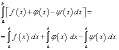 (42)
(42)
Theorem 5.If a segment of integration is divided into parts, then the definite integral over the entire segment is equal to the sum of definite integrals over its parts, i.e. If
![]() (43)
(43)
Theorem 6.When rearranging the limits of integration, the absolute value of the definite integral does not change, but only its sign changes, i.e.
![]() (44)
(44)
Theorem 7(mean value theorem). A definite integral is equal to the product of the length of the integration segment and the value of the integrand at some point inside it, i.e.
![]() (45)
(45)
Theorem 8.If the upper limit of integration is greater than the lower one and the integrand is non-negative (positive), then the definite integral is also non-negative (positive), i.e. If

Theorem 9.If the upper limit of integration is greater than the lower one and the functions and are continuous, then the inequality
can be integrated term by term, i.e.
![]() (46)
(46)
The properties of the definite integral make it possible to simplify the direct calculation of integrals.
Example 5. Calculate definite integral
![]()
Using Theorems 4 and 3, and when finding antiderivatives - table integrals (7) and (6), we obtain

Definite integral with variable upper limit
Let f(x) – continuous on the segment [ a, b] function, and F(x) is its antiderivative. Consider the definite integral
![]() (47)
(47)
and through t the integration variable is designated so as not to confuse it with the upper bound. When changing X the definite integral (47) also changes, i.e. it is a function of the upper limit of integration X, which we denote by F(X), i.e.
![]() (48)
(48)
Let us prove that the function F(X) is an antiderivative for f(x) = f(t). Indeed, differentiating F(X), we get

because F(x) – antiderivative for f(x), A F(a) is a constant value.
Function F(X) – one of the infinite number of antiderivatives for f(x), namely the one that x = a goes to zero. This statement is obtained if in equality (48) we put x = a and use Theorem 1 of the previous paragraph.
Calculation of definite integrals by the method of integration by parts and the method of change of variable
![]()
where, by definition, F(x) – antiderivative for f(x). If we change the variable in the integrand
then, in accordance with formula (16), we can write
In this expression
antiderivative function for
In fact, its derivative, according to rule of differentiation of complex functions, is equal

Let α and β be the values of the variable t, for which the function
takes values accordingly a And b, i.e.

But, according to the Newton-Leibniz formula, the difference F(b) – F(a) There is
Trapezoid method
Main article:Trapezoid method
If the function on each of the partial segments is approximated by a straight line passing through the finite values, then we obtain the trapezoidal method.
Area of the trapezoid on each segment:
Approximation error on each segment:
![]() Where
Where ![]()
The complete formula for trapezoids in the case of dividing the entire integration interval into segments of equal length:
 Where
Where
Trapezoid formula error:
![]() Where
Where ![]()
Simpson's method.
 Integrand f(x) is replaced by an interpolation polynomial of the second degree P(x)– a parabola passing through three nodes, for example, as shown in the figure ((1) – function, (2) – polynomial).
Let us consider two steps of integration ( h= const = x i+1 – x i), that is, three nodes x 0 , x 1 , x 2, through which we draw a parabola using Newton’s equation:
Let z = x - x 0,
Then
Now, using the obtained relation, we calculate the integral over this interval:

.
For uniform mesh And even number of steps n Simpson's formula takes the form:
Here ![]() , A
, A  under the assumption of continuity of the fourth derivative of the integrand.
[edit] Increased accuracy
Approximation of a function by a single polynomial over the entire integration interval, as a rule, leads to a large error in estimating the value of the integral.
To reduce the error, the integration segment is divided into parts and a numerical method is used to evaluate the integral on each of them.
As the number of partitions tends to infinity, the estimate of the integral tends to its true value for analytical functions for any numerical method.
The above methods allow a simple procedure of halving the step, with each step requiring the function values to be calculated only at the newly added nodes. To estimate the calculation error, Runge's rule is used.
Application of Runge's rule
edit]Assessing the accuracy of calculating a certain integral
The integral is calculated using the selected formula (rectangles, trapezoids, Simpson parabolas) with the number of steps equal to n, and then with the number of steps equal to 2n. The error in calculating the value of the integral with a number of steps equal to 2n is determined by the Runge formula:
, for formulas of rectangles and trapezoids, and for Simpson's formula.
Thus, the integral is calculated for successive values of the number of steps, where n 0 is the initial number of steps. The calculation process ends when the condition is satisfied for the next value N, where ε is the specified accuracy.
Features of error behavior.
It would seem, why analyze different integration methods if we can achieve high accuracy simply by reducing the integration step size. However, consider the graph of the behavior of the posterior error R results of numerical calculation depending on  and from the number n interval partitions (that is, at step . In section (1), the error decreases due to a decrease in step h. But in section (2), the computational error begins to dominate, accumulating as a result of numerous arithmetic operations. Thus, each method has its own Rmin, which depends on many factors, but primarily on the a priori value of the method error R.
Romberg's clarifying formula.
Romberg's method consists of sequentially refining the value of the integral with a multiple increase in the number of partitions. The formula of trapezoids with uniform steps can be taken as a base h.
Let us denote the integral with the number of partitions n= 1 as ![]() .
.
Reducing the step by half, we get ![]() .
.
If we successively reduce the step by 2 n times, we obtain a recurrence relation for calculating .


