The distribution series is given. Law of probability distribution of a discrete random variable

In applications of probability theory, the quantitative characteristics of the experiment are of primary importance. A quantity that can be quantitatively determined and which, as a result of an experiment, can take on different values depending on the case is called random variable.

Examples of random variables:

1. The number of times an even number of points appears in ten throws of a die.

2. The number of hits on the target by a shooter who fires a series of shots.

3. The number of fragments of an exploding shell.

In each of the examples given, the random variable can only take on isolated values, that is, values that can be numbered using a natural series of numbers.

Such a random variable, the possible values of which are individual isolated numbers, which this variable takes with certain probabilities, is called discrete.

The number of possible values of a discrete random variable can be finite or infinite (countable).

Law of distribution A discrete random variable is a list of its possible values and their corresponding probabilities. The distribution law of a discrete random variable can be specified in the form of a table (probability distribution series), analytically and graphically (probability distribution polygon).

When carrying out this or that experiment, it becomes necessary to evaluate the value being studied “on average.” The role of the average value of a random variable is played by a numerical characteristic called mathematical expectation, which is determined by the formula

Where x 1 , x 2 ,.. , x n– random variable values X, A p 1 ,p 2 , ... , p n– the probabilities of these values (note that p 1 + p 2 +…+ p n = 1).

Example. Shooting is carried out at the target (Fig. 11).

A hit in I gives three points, in II – two points, in III – one point. The number of points scored in one shot by one shooter has a distribution law of the form

To compare the skill of shooters, it is enough to compare the average values of the points scored, i.e. mathematical expectations M(X) And M(Y):

M(X) = 1 0,4 + 2  0,2 + 3  0,4 = 2,0,

M(Y) = 1 0,2 + 2  0,5 + 3  0,3 = 2,1.

The second shooter gives on average a slightly higher number of points, i.e. it will give better results when fired repeatedly.

Let us note the properties of the mathematical expectation:

1. The mathematical expectation of a constant value is equal to the constant itself:

M(C) =C.

2. The mathematical expectation of the sum of random variables is equal to the sum of the mathematical expectations of the terms:

M =(X 1 + X 2 +…+ X n)= M(X 1)+ M(X 2)+…+ M(X n).

3. The mathematical expectation of the product of mutually independent random variables is equal to the product of the mathematical expectations of the factors

M(X 1 X 2 … X n) = M(X 1)M(X 2)… M(X n).

4. The mathematical negation of the binomial distribution is equal to the product of the number of trials and the probability of an event occurring in one trial (task 4.6).

M(X) = pr.

To assess how a random variable “on average” deviates from its mathematical expectation, i.e. In order to characterize the spread of values of a random variable in probability theory, the concept of dispersion is used.

Variance random variable X is called the mathematical expectation of the squared deviation:

D(X) = M[(X - M(X)) 2 ].

Dispersion is a numerical characteristic of the dispersion of a random variable. From the definition it is clear that the smaller the dispersion of a random variable, the more closely its possible values are located around the mathematical expectation, that is, the better the values of the random variable are characterized by its mathematical expectation.

From the definition it follows that the variance can be calculated using the formula

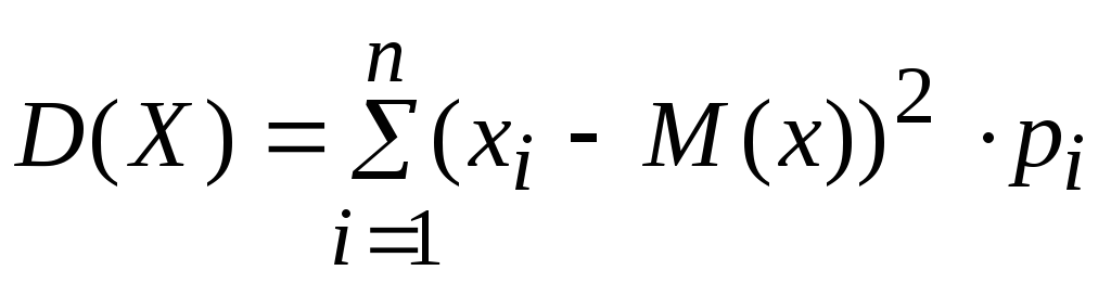It is convenient to calculate the variance using another formula:

D(X) = M(X 2) - (M(X)) 2 .

The dispersion has the following properties:

1. The variance of the constant is zero:

D(C) = 0.

2. The constant factor can be taken out of the dispersion sign by squaring it:

D(CX) = C 2 D(X).

3. The variance of the sum of independent random variables is equal to the sum of the variance of the terms:

D(X 1 + X 2 + X 3 +…+ X n)= D(X 1)+ D(X 2)+…+ D(X n)

4. The variance of the binomial distribution is equal to the product of the number of trials and the probability of the occurrence and non-occurrence of an event in one trial:

D(X) = npq.

In probability theory, a numerical characteristic equal to the square root of the variance of a random variable is often used. This numerical characteristic is called the mean square deviation and is denoted by the symbol

It characterizes the approximate size of the deviation of a random variable from its average value and has the same dimension as the random variable.

4.1. The shooter fires three shots at the target. The probability of hitting the target with each shot is 0.3.

Construct a distribution series for the number of hits.

Solution. The number of hits is a discrete random variable X. Each value x n random variable X corresponds to a certain probability P n .

The distribution law of a discrete random variable in this case can be specified near distribution.

In this problem X takes values 0, 1, 2, 3. According to Bernoulli's formula

Let's find the probabilities of possible values of a random variable:

R 3 (0) = (0,7) 3 = 0,343,

R 3 (1) =0,3(0,7) 2 = 0,441,

R 3 (2) =(0,3) 2 0,7 = 0,189,

R 3 (3) = (0,3) 3 = 0,027.

By arranging the values of the random variable X in increasing order, we obtain the distribution series:

X n

Note that the amount

means the probability that the random variable X will take at least one value from among the possible ones, and this event is reliable, therefore

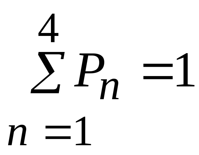4.2 .There are four balls in the urn with numbers from 1 to 4. Two balls are taken out. Random value X– the sum of the ball numbers. Construct a distribution series of a random variable X.

Solution. Random variable values X are 3, 4, 5, 6, 7. Let's find the corresponding probabilities. Random variable value 3 X can be accepted in the only case when one of the selected balls has the number 1, and the other 2. The number of possible test outcomes is equal to the number of combinations of four (the number of possible pairs of balls) of two.

Using the classical probability formula we get

Likewise,

R(X= 4) =R(X= 6) =R(X= 7) = 1/6.

The sum 5 can appear in two cases: 1 + 4 and 2 + 3, so

X has the form:

Find the distribution function F(x) random variable X and plot it. Calculate for X its mathematical expectation and variance.

Solution. The distribution law of a random variable can be specified by the distribution function

F(x) = P(X x).

Distribution function F(x) is a non-decreasing, left-continuous function defined on the entire number line, while

F (- )= 0,F (+ )= 1.

For a discrete random variable, this function is expressed by the formula

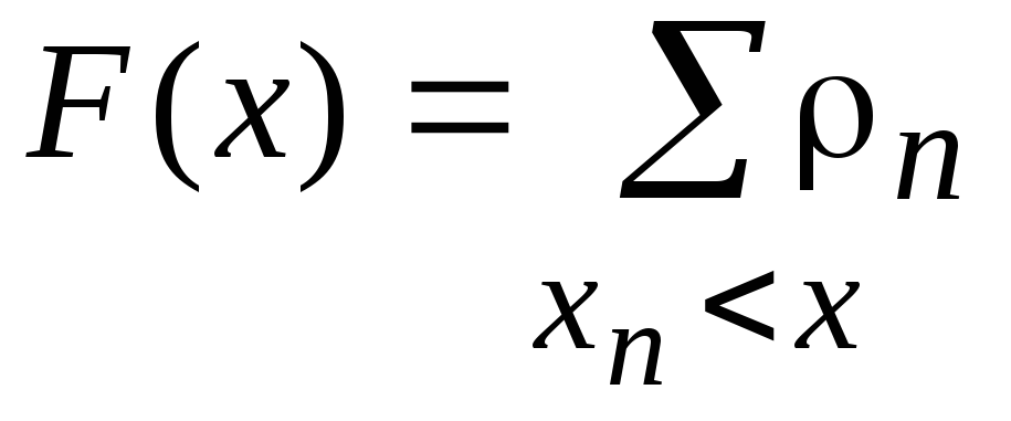Therefore in this case

Distribution function graph F(x) is a stepped line (Fig. 12)

	F(x)

Expected valueM(X) is the weighted arithmetic average of the values X 1 , X 2 ,……X n random variable X with scales ρ 1, ρ 2, …… , ρ n and is called the mean value of the random variable X. According to the formula

M(X)= x 1 ρ 1 + x 2 ρ 2 +……+ x n ρ n

M(X) = 3·0.14+5·0.2+7·0.49+11·0.17 = 6.72.

Dispersion characterizes the degree of dispersion of the values of a random variable from its average value and is denoted D(X):

D(X)=M[(HM(X)) 2 ]= M(X 2) –[M(X)] 2 .

For a discrete random variable, the variance has the form

or it can be calculated using the formula

Substituting the numerical data of the problem into the formula, we get:

M(X 2) = 3 2 ∙ 0,14+5 2 ∙ 0,2+7 2 ∙ 0,49+11 2 ∙ 0,17 = 50,84

D(X) = 50,84-6,72 2 = 5,6816.

4.4. Two dice are rolled twice at the same time. Write the binomial law of distribution of a discrete random variable X- the number of occurrences of an even total number of points on two dice.

Solution. Let us introduce a random event

A= (two dice with one throw resulted in a total of even number of points).

Using the classical definition of probability we find

R(A)= ,

Where n - the number of possible test outcomes is found by the rule

multiplication:

n = 6∙6 =36,

m - number of people favoring the event A outcomes - equal

m= 3∙6=18.

Thus, the probability of success in one trial is

ρ = P(A)= 1/2.

The problem is solved using a Bernoulli test scheme. One challenge here will be rolling two dice once. Number of such tests n = 2. Random variable X takes values 0, 1, 2 with probabilities

R 2 (0) =,R 2 (1) =∙,R 2 (2) =

The required binomial distribution of a random variable X can be represented as a distribution series:

X n
ρ n

4.5 . In a batch of six parts there are four standard ones. Three parts were selected at random. Construct a probability distribution of a discrete random variable X– the number of standard parts among those selected and find its mathematical expectation.

Solution. Random variable values X are the numbers 0,1,2,3. It's clear that R(X=0)=0, since there are only two non-standard parts.

R(X=1) =
=1/5,

R(X= 2) =
= 3/5,

R(X=3) =
= 1/5.

Distribution law of a random variable X Let's present it in the form of a distribution series:

X n
ρ n

Expected value

M(X)=1 ∙ 1/5+2 ∙ 3/5+3 ∙ 1/5=2.

4.6 . Prove that the mathematical expectation of a discrete random variable X- number of occurrences of the event A V n independent trials, in each of which the probability of an event occurring is equal to ρ – equal to the product of the number of trials by the probability of the occurrence of an event in one trial, that is, to prove that the mathematical expectation of the binomial distribution

M(X) =n . ρ ,

and dispersion

D(X) =n.p. .

Solution. Random value X can take values 0, 1, 2..., n. Probability R(X= k) is found using Bernoulli’s formula:

R(X=k)= R n(k)= ρ To (1-ρ ) n- To

Distribution series of a random variable X has the form:

X n
ρ n	q n	ρq n- 1	ρq n- 2		ρ n

Where q= 1- ρ .

For the mathematical expectation we have the expression:

M(X)=ρq n - 1 +2 ρ 2 q n - 2 +…+.n ρ n

In the case of one test, that is, with n= 1 for random variable X 1 – number of occurrences of the event A- the distribution series has the form:

X n
ρ n

M(X 1)= 0∙q + 1 ∙ p = p

D(X 1) = p – p 2 = p(1- p) = pq.

If X k – number of occurrences of the event A in which test, then R(X To)= ρ And

X=X 1 +X 2 +….+X n .

From here we get

M(X)=M(X 1 )+M(X 2)+ … +M(X n)= nρ,

D(X)=D(X 1)+D(X 2)+ ... +D(X n)=npq.

4.7. The quality control department checks products for standardness. The probability that the product is standard is 0.9. Each batch contains 5 products. Find the mathematical expectation of a discrete random variable X- the number of batches, each of which will contain 4 standard products - if 50 batches are subject to inspection.

Solution. The probability that there will be 4 standard products in each randomly selected batch is constant; let's denote it by ρ .Then the mathematical expectation of the random variable X equals M(X)= 50∙ρ.

Let's find the probability ρ according to Bernoulli's formula:

ρ=P 5 (4)== 0,94∙0,1=0,32.

M(X)= 50∙0,32=16.

4.8 . Three dice are thrown. Find the mathematical expectation of the sum of the dropped points.

Solution. You can find the distribution of a random variable X- the sum of the dropped points and then its mathematical expectation. However, this path is too cumbersome. It is easier to use another technique, representing a random variable X, the mathematical expectation of which needs to be calculated, in the form of a sum of several simpler random variables, the mathematical expectation of which is easier to calculate. If the random variable X i is the number of points rolled on i– th bones ( i= 1, 2, 3), then the sum of points X will be expressed in the form

X = X 1 + X 2 + X 3 .

To calculate the mathematical expectation of the original random variable, all that remains is to use the property of mathematical expectation

M(X 1 + X 2 + X 3 )= M(X 1 )+ M(X 2)+ M(X 3 ).

It's obvious that

R(X i = K)= 1/6, TO= 1, 2, 3, 4, 5, 6, i= 1, 2, 3.

Therefore, the mathematical expectation of the random variable X i looks like

M(X i) = 1/6∙1 + 1/6∙2 +1/6∙3 + 1/6∙4 + 1/6∙5 + 1/6∙6 = 7/2,

M(X) = 3∙7/2 = 10,5.

4.9. Determine the mathematical expectation of the number of devices that failed during testing if:

a) the probability of failure for all devices is the same R, and the number of devices under test is equal to n;

b) probability of failure for i – of the device is equal to p i , i= 1, 2, … , n.

Solution. Let the random variable X is the number of failed devices, then

X = X 1 + X 2 + … + X n ,

X i =

It's clear that

R(X i = 1)= R i , R(X i = 0)= 1– R i ,i= 1, 2, … ,n.

M(X i)= 1∙R i + 0∙(1-R i)=P i ,

M(X)=M(X 1)+M(X 2)+ … +M(X n)=P 1 +P 2 + … + P n .

In case “a” the probability of device failure is the same, that is

R i =p,i= 1, 2, … ,n.

M(X)= n.p..

This answer could be obtained immediately if we notice that the random variable X has a binomial distribution with parameters ( n, p).

4.10. Two dice are thrown simultaneously twice. Write the binomial law of distribution of a discrete random variable X - the number of rolls of an even number of points on two dice.

Solution. Let

A=(rolling an even number on the first die),

B =(rolling an even number on the second dice).

Getting an even number on both dice in one throw is expressed by the product AB. Then

R (AB) = R(A)∙R(IN) =
.

The result of the second throw of two dice does not depend on the first, so Bernoulli's formula applies when

n = 2,p = 1/4, q = 1– p = 3/4.

Random value X can take values 0, 1, 2 , the probability of which can be found using Bernoulli’s formula:

R(X= 0)= P 2 (0) = q 2 = 9/16,

R(X= 1)= P 2 (1)= C ,R∙q = 6/16,

R(X= 2)= P 2 (2)= C , R 2 = 1/16.

Distribution series of a random variable X:

4.11. The device consists of a large number of independently operating elements with the same very small probability of failure of each element over time t. Find the average number of refusals over time t elements, if the probability that at least one element will fail during this time is 0.98.

Solution. Number of people who refused over time t elements – random variable X, which is distributed according to Poisson's law, since the number of elements is large, the elements work independently and the probability of failure of each element is small. Average number of occurrences of an event in n tests equals

M(X) = n.p..

Since the probability of failure TO elements from n expressed by the formula

R n (TO)
,

where  = n.p., then the probability that not a single element will fail during the time t we get at K = 0:

R n (0)= e -  .

Therefore, the probability of the opposite event is in time t at least one element fails – equal to 1 - e -  . According to the conditions of the problem, this probability is 0.98. From Eq.

1 - e -  = 0,98,

e -  = 1 – 0,98 = 0,02,

from here  = -ln 0,02  4.

So, in time t operation of the device, on average 4 elements will fail.

4.12 . The dice are rolled until a “two” comes up. Find the average number of throws.

Solution. Let's introduce a random variable X– the number of tests that must be performed until the event of interest to us occurs. The probability that X= 1 is equal to the probability that during one throw of the dice a “two” will appear, i.e.

R(X= 1) = 1/6.

Event X= 2 means that on the first test the “two” did not come up, but on the second it did. Probability of event X= 2 is found by the rule of multiplying the probabilities of independent events:

R(X= 2) = (5/6)∙(1/6)

Likewise,

R(X= 3) = (5/6) 2 ∙1/6, R(X= 4) = (5/6) 2 ∙1/6

etc. We obtain a series of probability distributions:


					(5/6) To ∙1/6

The average number of throws (trials) is the mathematical expectation

M(X) = 1∙1/6 + 2∙5/6∙1/6 + 3∙(5/6) 2 ∙1/6 + … + TO (5/6) TO -1 ∙1/6 + … =

1/6∙(1+2∙5/6 +3∙(5/6) 2 + … + TO (5/6) TO -1 + …)

Let's find the sum of the series:

TOg TO -1 = (g TO) g 
.

Hence,

M(X) = (1/6) (1/ (1 – 5/6) 2 = 6.

Thus, you need to make an average of 6 throws of the dice until a “two” comes up.

4.13. Independent tests are carried out with the same probability of occurrence of the event A in every test. Find the probability of an event occurring A, if the variance of the number of occurrences of an event in three independent trials is 0.63 .

Solution. The number of occurrences of an event in three trials is a random variable X, distributed according to the binomial law. The variance of the number of occurrences of an event in independent trials (with the same probability of occurrence of the event in each trial) is equal to the product of the number of trials by the probabilities of the occurrence and non-occurrence of the event (problem 4.6)

D(X) = npq.

By condition n = 3, D(X) = 0.63, so you can R find from equation

0,63 = 3∙R(1-R),

which has two solutions R 1 = 0.7 and R 2 = 0,3.

On this page we have collected examples of educational solutions problems about discrete random variables. This is a fairly extensive section: various distribution laws (binomial, geometric, hypergeometric, Poisson and others), properties and numerical characteristics are studied; for each distribution series, graphical representations can be built: polygon (polygon) of probabilities, distribution function.

Below you will find examples of decisions about discrete random variables, in which you need to apply knowledge from previous sections of probability theory to draw up a distribution law, and then calculate the mathematical expectation, dispersion, standard deviation, construct a distribution function, answer questions about the DSV, etc. P.

Examples for popular probability distribution laws:

Calculators for DSV characteristics

Calculation of mathematical expectation, dispersion and standard deviation of DSV.

Solved problems about DSV

Distributions close to geometric

Task 1. There are 4 traffic lights along the path of the car, each of which prohibits further movement of the car with a probability of 0.5. Find the distribution series of the number of traffic lights passed by the car before the first stop. What are the mathematical expectation and variance of this random variable?

Task 2. The hunter shoots at the game until the first hit, but manages to fire no more than four shots. Draw up a distribution law for the number of misses if the probability of hitting the target with one shot is 0.7. Find the variance of this random variable.

Task 3. The shooter, having 3 cartridges, shoots at the target until the first hit. The hit probabilities for the first, second and third shots are 0.6, 0.5, 0.4, respectively. S.V. $\xi$ - number of remaining cartridges. Compile a distribution series of a random variable, find the mathematical expectation, variance, standard deviation of the random variable, construct the distribution function of the random variable, find $P(|\xi-m| \le \sigma$.

Task 4. The box contains 7 standard and 3 defective parts. They take out the parts sequentially until the standard one appears, without returning them back. $\xi$ is the number of defective parts retrieved.
Draw up a distribution law for a discrete random variable $\xi$, calculate its mathematical expectation, variance, standard deviation, draw a distribution polygon and a graph of the distribution function.

Tasks with independent events

Task 5. 3 students appeared for the re-exam in probability theory. The probability that the first person will pass the exam is 0.8, the second - 0.7, and the third - 0.9. Find the distribution series of the random variable $\xi$ of the number of students who passed the exam, plot the distribution function, find $M(\xi), D(\xi)$.

Task 6. The probability of hitting the target with one shot is 0.8 and decreases with each shot by 0.1. Draw up a distribution law for the number of hits on a target if three shots are fired. Find the expected value, variance and S.K.O. this random variable. Draw a graph of the distribution function.

Task 7. 4 shots are fired at the target. The probability of a hit increases as follows: 0.2, 0.4, 0.6, 0.7. Find the law of distribution of the random variable $X$ - the number of hits. Find the probability that $X \ge 1$.

Task 8. Two symmetrical coins are tossed and the number of coats of arms on both top sides of the coins is counted. We consider a discrete random variable $X$ - the number of coats of arms on both coins. Write down the distribution law of the random variable $X$, find its mathematical expectation.

1. Law of probability distribution of a discrete random variable.

A discrete random variable $X$ can take values $x_1,\dots ,\ x_n$ with probabilities $p\left(x_1\right),\ \dots ,\ p\left(x_n\right)$. The correspondence between these values and their probabilities is called law of distribution of a discrete random variable. As a rule, this correspondence is specified using a table, the first line of which indicates the values $x_1,\dots ,\ x_n$, and the second line contains the probabilities $p_1,\dots ,\ p_n$ corresponding to these values.

$\begin(array)(|c|c|)
\hline
X_i & x_1 & x_2 & \dots & x_n \\
\hline
p_i & p_1 & p_2 & \dots & p_n \\
\hline
\end(array)$

Example 2 . Let the random variable $X$ be the number of points rolled when tossing a die. Such a random variable $X$ can take the following values: $1,\ 2,\ 3,\ 4,\ 5,\ 6$. The probabilities of all these values are equal to $1/6$. Then the law of probability distribution of the random variable $X$:

$\begin(array)(|c|c|)
\hline
1 & 2 & 3 & 4 & 5 & 6 \\
\hline

\hline
\end(array)$

Comment. Since in the distribution law of a discrete random variable $X$ the events $1,\ 2,\ \dots ,\ 6$ form a complete group of events, then the sum of the probabilities must be equal to one, that is, $\sum(p_i)=1$.

2. Mathematical expectation of a discrete random variable.

Mathematical expectation of a random variable sets its “central” meaning. For a discrete random variable, the mathematical expectation is calculated as the sum of the products of the values $x_1,\dots ,\ x_n$ and the probabilities $p_1,\dots ,\ p_n$ corresponding to these values, that is: $M\left(X\right)=\sum ^n_(i=1)(p_ix_i)$. In English-language literature, another notation $E\left(X\right)$ is used.

Properties of mathematical expectation$M\left(X\right)$:

$M\left(X\right)$ lies between the smallest and largest values of the random variable $X$.
The mathematical expectation of a constant is equal to the constant itself, i.e. $M\left(C\right)=C$.
The constant factor can be taken out of the sign of the mathematical expectation: $M\left(CX\right)=CM\left(X\right)$.
The mathematical expectation of the sum of random variables is equal to the sum of their mathematical expectations: $M\left(X+Y\right)=M\left(X\right)+M\left(Y\right)$.
The mathematical expectation of the product of independent random variables is equal to the product of their mathematical expectations: $M\left(XY\right)=M\left(X\right)M\left(Y\right)$.

Example 3 . Let's find the mathematical expectation of the random variable $X$ from example $2$.

$$M\left(X\right)=\sum^n_(i=1)(p_ix_i)=1\cdot ((1)\over (6))+2\cdot ((1)\over (6) )+3\cdot ((1)\over (6))+4\cdot ((1)\over (6))+5\cdot ((1)\over (6))+6\cdot ((1 )\over (6))=3.5.$$

We can notice that $M\left(X\right)$ lies between the smallest ($1$) and largest ($6$) values of the random variable $X$.

Example 4 . It is known that the mathematical expectation of the random variable $X$ is equal to $M\left(X\right)=2$. Find the mathematical expectation of the random variable $3X+5$.

Using the above properties, we get $M\left(3X+5\right)=M\left(3X\right)+M\left(5\right)=3M\left(X\right)+5=3\cdot 2 +5=$11.

Example 5 . It is known that the mathematical expectation of the random variable $X$ is equal to $M\left(X\right)=4$. Find the mathematical expectation of the random variable $2X-9$.

Using the above properties, we get $M\left(2X-9\right)=M\left(2X\right)-M\left(9\right)=2M\left(X\right)-9=2\cdot 4 -9=-1$.

3. Dispersion of a discrete random variable.

Possible values of random variables with equal mathematical expectations can disperse differently around their average values. For example, in two student groups the average score for the exam in probability theory turned out to be 4, but in one group everyone turned out to be good students, and in the other group there were only C students and excellent students. Therefore, there is a need for a numerical characteristic of a random variable that would show the spread of the values of the random variable around its mathematical expectation. This characteristic is dispersion.

Variance of a discrete random variable$X$ is equal to:

$$D\left(X\right)=\sum^n_(i=1)(p_i(\left(x_i-M\left(X\right)\right))^2).\ $$

In English literature the notation $V\left(X\right),\ Var\left(X\right)$ is used. Very often the variance $D\left(X\right)$ is calculated using the formula $D\left(X\right)=\sum^n_(i=1)(p_ix^2_i)-(\left(M\left(X \right)\right))^2$.

Dispersion properties$D\left(X\right)$:

The variance is always greater than or equal to zero, i.e. $D\left(X\right)\ge 0$.
The variance of the constant is zero, i.e. $D\left(C\right)=0$.
The constant factor can be taken out of the sign of the dispersion provided that it is squared, i.e. $D\left(CX\right)=C^2D\left(X\right)$.
The variance of the sum of independent random variables is equal to the sum of their variances, i.e. $D\left(X+Y\right)=D\left(X\right)+D\left(Y\right)$.
The variance of the difference between independent random variables is equal to the sum of their variances, i.e. $D\left(X-Y\right)=D\left(X\right)+D\left(Y\right)$.

Example 6 . Let's calculate the variance of the random variable $X$ from example $2$.

$$D\left(X\right)=\sum^n_(i=1)(p_i(\left(x_i-M\left(X\right)\right))^2)=((1)\over (6))\cdot (\left(1-3.5\right))^2+((1)\over (6))\cdot (\left(2-3.5\right))^2+ \dots +((1)\over (6))\cdot (\left(6-3.5\right))^2=((35)\over (12))\approx 2.92.$$

Example 7 . It is known that the variance of the random variable $X$ is equal to $D\left(X\right)=2$. Find the variance of the random variable $4X+1$.

Using the above properties, we find $D\left(4X+1\right)=D\left(4X\right)+D\left(1\right)=4^2D\left(X\right)+0=16D\ left(X\right)=16\cdot 2=32$.

Example 8 . It is known that the variance of the random variable $X$ is equal to $D\left(X\right)=3$. Find the variance of the random variable $3-2X$.

Using the above properties, we find $D\left(3-2X\right)=D\left(3\right)+D\left(2X\right)=0+2^2D\left(X\right)=4D\ left(X\right)=4\cdot 3=12$.

4. Distribution function of a discrete random variable.

The method of representing a discrete random variable in the form of a distribution series is not the only one, and most importantly, it is not universal, since a continuous random variable cannot be specified using a distribution series. There is another way to represent a random variable - the distribution function.

Distribution function random variable $X$ is called a function $F\left(x\right)$, which determines the probability that the random variable $X$ will take a value less than some fixed value $x$, that is, $F\left(x\right )=P\left(X< x\right)$

Properties of the distribution function:

$0\le F\left(x\right)\le 1$.
The probability that the random variable $X$ will take values from the interval $\left(\alpha ;\ \beta \right)$ is equal to the difference between the values of the distribution function at the ends of this interval: $P\left(\alpha< X < \beta \right)=F\left(\beta \right)-F\left(\alpha \right)$
$F\left(x\right)$ - non-decreasing.
$(\mathop(lim)_(x\to -\infty ) F\left(x\right)=0\ ),\ (\mathop(lim)_(x\to +\infty ) F\left(x \right)=1\ )$.

Example 9 . Let us find the distribution function $F\left(x\right)$ for the distribution law of the discrete random variable $X$ from example $2$.

$\begin(array)(|c|c|)
\hline
1 & 2 & 3 & 4 & 5 & 6 \\
\hline
1/6 & 1/6 & 1/6 & 1/6 & 1/6 & 1/6 \\
\hline
\end(array)$

If $x\le 1$, then, obviously, $F\left(x\right)=0$ (including for $x=1$ $F\left(1\right)=P\left(X< 1\right)=0$).

If $1< x\le 2$, то $F\left(x\right)=P\left(X=1\right)=1/6$.

If $2< x\le 3$, то $F\left(x\right)=P\left(X=1\right)+P\left(X=2\right)=1/6+1/6=1/3$.

If $3< x\le 4$, то $F\left(x\right)=P\left(X=1\right)+P\left(X=2\right)+P\left(X=3\right)=1/6+1/6+1/6=1/2$.

If $4< x\le 5$, то $F\left(X\right)=P\left(X=1\right)+P\left(X=2\right)+P\left(X=3\right)+P\left(X=4\right)=1/6+1/6+1/6+1/6=2/3$.

If $5< x\le 6$, то $F\left(x\right)=P\left(X=1\right)+P\left(X=2\right)+P\left(X=3\right)+P\left(X=4\right)+P\left(X=5\right)=1/6+1/6+1/6+1/6+1/6=5/6$.

If $x > 6$, then $F\left(x\right)=P\left(X=1\right)+P\left(X=2\right)+P\left(X=3\right) +P\left(X=4\right)+P\left(X=5\right)+P\left(X=6\right)=1/6+1/6+1/6+1/6+ 1/6+1/6=1$.

So $F(x)=\left\(\begin(matrix)
0,\ at\ x\le 1,\\
1/6,at\ 1< x\le 2,\\
1/3,\ at\ 2< x\le 3,\\
1/2,at\ 3< x\le 4,\\
2/3,\ at\ 4< x\le 5,\\
5/6,\ at\ 4< x\le 5,\\
1,\ for\ x > 6.
\end(matrix)\right.$

One of the most important concepts in probability theory is the concept random variable.

Random called size, which as a result of testing takes on certain possible values that are unknown in advance and depend on random reasons that cannot be taken into account in advance.

Random variables are designated by capital letters of the Latin alphabet X, Y, Z etc. or in capital letters of the Latin alphabet with a right lower index, and the values that random variables can take - in the corresponding small letters of the Latin alphabet x, y, z etc.

The concept of a random variable is closely related to the concept of a random event. Connection with a random event lies in the fact that the adoption of a certain numerical value by a random variable is a random event characterized by probability .

In practice, there are two main types of random variables:

1. Discrete random variables;

2. Continuous random variables.

A random variable is a numerical function of random events.

For example, a random variable is the number of points obtained when throwing a die, or the height of a student randomly selected from a study group.

Discrete random variables are called random variables that take only values distant from each other that can be listed in advance.

Law of distribution(distribution function and distribution series or probability density) completely describe the behavior of a random variable. But in a number of problems, it is enough to know some numerical characteristics of the quantity under study (for example, its average value and possible deviation from it) in order to answer the question posed. Let's consider the main numerical characteristics of discrete random variables.

Distribution law of a discrete random variable every relation is called , establishing a connection between possible values of a random variable and their corresponding probabilities .

The distribution law of a random variable can be represented as tables:

			…	…
			…	…

The sum of the probabilities of all possible values of a random variable is equal to one, i.e.

The distribution law can be depicted graphically: the possible values of a random variable are plotted along the abscissa axis, and the probabilities of these values are plotted along the ordinate axis; the resulting points are connected by segments. The constructed polyline is called distribution polygon.

Example. A hunter with 4 cartridges shoots at the game until he makes the first hit or uses up all the cartridges. The probability of hitting on the first shot is 0.7, with each subsequent shot it decreases by 0.1. Draw up a distribution law for the number of cartridges spent by a hunter.

Solution. Since a hunter, having 4 cartridges, can fire four shots, then the random variable X- the number of cartridges spent by the hunter can take values 1, 2, 3, 4. To find the corresponding probabilities, we introduce the events:

- “hit with i- oh shot”, ;

- “miss when i- om shot”, and the events and are pairwise independent.

According to the problem conditions we have:

Using the multiplication theorem for independent events and the addition theorem for incompatible events, we find:

(the hunter hit the target with the first shot);

(the hunter hit the target with the second shot);

(the hunter hit the target with the third shot);

(the hunter hit the target with the fourth shot or missed all four times).

Check: - true.

Thus, the law of distribution of a random variable X has the form:


	0,7	0,18	0,06	0,06

Example. A worker operates three machines. The probability that within an hour the first machine will not require adjustment is 0.9, the second - 0.8, the third - 0.7. Draw up a distribution law for the number of machines that will require adjustment within an hour.

Solution. Random value X- the number of machines that will require adjustment within an hour can take values 0,1, 2, 3. To find the corresponding probabilities, we introduce the events:

- “i- the machine will require adjustment within an hour”, ;

- “i- the machine will not require adjustment within an hour.”

According to the problem conditions we have:

, .

Discrete random Variables are random variables that take only values that are distant from each other and that can be listed in advance.
Law of distribution
The distribution law of a random variable is a relationship that establishes a connection between the possible values of a random variable and their corresponding probabilities.
The distribution series of a discrete random variable is the list of its possible values and the corresponding probabilities.
The distribution function of a discrete random variable is the function:
,
determining for each value of the argument x the probability that the random variable X will take a value less than this x.

Expectation of a discrete random variable
,
where is the value of a discrete random variable; - the probability of a random variable accepting X values.
If a random variable takes a countable set of possible values, then:
.
Mathematical expectation of the number of occurrences of an event in n independent trials:
,

Dispersion and standard deviation of a discrete random variable
Dispersion of a discrete random variable:
or .
Variance of the number of occurrences of an event in n independent trials
,
where p is the probability of the event occurring.
Standard deviation of a discrete random variable:
.

Example 1
Draw up a law of probability distribution for a discrete random variable (DRV) X – the number of k occurrences of at least one “six” in n = 8 throws of a pair of dice. Construct a distribution polygon. Find the numerical characteristics of the distribution (distribution mode, mathematical expectation M(X), dispersion D(X), standard deviation s(X)). Solution: Let us introduce the notation: event A – “when throwing a pair of dice, a six appears at least once.” To find the probability P(A) = p of event A, it is more convenient to first find the probability P(Ā) = q of the opposite event Ā - “when throwing a pair of dice, a six never appeared.”
Since the probability of a “six” not appearing when throwing one die is 5/6, then according to the probability multiplication theorem
P(Ā) = q = = .
Respectively,
P(A) = p = 1 – P(Ā) = .
The tests in the problem follow the Bernoulli scheme, so d.s.v. magnitude X- number k the occurrence of at least one six when throwing two dice obeys the binomial law of probability distribution:

where = is the number of combinations of n By k.

The calculations carried out for this problem can be conveniently presented in the form of a table:
Probability distribution d.s.v. X º k (n = 8; p = ; q = )

k

Pn(k)

Polygon (polygon) of probability distribution of a discrete random variable X shown in the figure:

Rice. Probability distribution polygon d.s.v. X=k.
The vertical line shows the mathematical expectation of the distribution M(X).

Let us find the numerical characteristics of the probability distribution of d.s.v. X. The distribution mode is 2 (here P 8(2) = 0.2932 maximum). The mathematical expectation by definition is equal to:
M(X) = = 2,4444,
Where xk = k– value taken by d.s.v. X. Variance D(X) we find the distribution using the formula:
D(X) = = 4,8097.
Standard deviation (RMS):
s( X) = = 2,1931.

Example2
Discrete random variable X given by the distribution law

Find the distribution function F(x) and plot it.

Solution. If , then (third property).
If, then. Really, X can take the value 1 with probability 0.3.
If, then. Indeed, if it satisfies the inequality
, then equals the probability of an event that can occur when X will take the value 1 (the probability of this event is 0.3) or the value 4 (the probability of this event is 0.1). Since these two events are incompatible, then, according to the addition theorem, the probability of an event is equal to the sum of the probabilities 0.3 + 0.1 = 0.4. If, then. Indeed, the event is certain, therefore its probability is equal to one. So, the distribution function can be written analytically as follows:

Graph of this function:
Let us find the probabilities corresponding to these values. By condition, the probabilities of failure of the devices are equal: then the probabilities that the devices will work during the warranty period are equal:

The distribution law has the form: