What are you looking at now? If you are not from parallel universe, where everyone is sitting behind vector monitors, then in front of you raster image. Look at this strip: /. If you move closer to the monitor, you can see pixelated steps that are trying to pretend to be a vector line. There are a whole bunch of different rasterization algorithms for this purpose, but I would like to talk about the Bresenham algorithm and the Y algorithm, which find an approximation of a vector segment in raster coordinates.
I encountered the problem of rasterization while working on a procedural generator of building plans. I needed to represent the walls of the room as cells of a two-dimensional array. Similar problems can be encountered in physics calculations, path finding algorithms, or lighting calculations if space partitioning is used. Who would have thought that familiarity with rasterization algorithms could one day come in handy?
The operating principle of Bresenham's algorithm is very simple. Take a segment and its initial coordinate x. To the x in the cycle we add one at a time towards the end of the segment. At each step, the error is calculated - the distance between the real coordinate y at this location and the nearest grid cell. If the error does not exceed half the height of the cell, then it is filled. That's the whole algorithm.
This was the essence of the algorithm, in reality everything looks like this. First, the slope is calculated (y1 - y0)/(x1 - x0). Error value at the starting point of the segment (0,0) accepted equal to zero and the first cell is filled. At the next step, the slope is added to the error and its value is analyzed if the error is less 0.5 , then the cell is filled (x0+1, y0), if more, then the cell is filled (x0+1, y0+1) and one is subtracted from the error value. In the picture below yellow the line before rasterization is shown, green and red - the distance to the nearest cells. The slope is equal to one sixth, at the first step the error becomes equal to the slope, which is less 0.5 , which means the ordinate remains the same. Towards the middle of the line, the error crosses the line, one is subtracted from it, and the new pixel rises higher. And so on until the end of the segment.

One more nuance. If the projection of a segment onto the axis x less projection on the axis y or the beginning and end of the segment are swapped, then the algorithm will not work. To prevent this from happening, you need to check the direction of the vector and its slope, and then, if necessary, swap the coordinates of the segment, rotate the axes, and, ultimately, reduce everything to one or at least two cases. The main thing is not to forget to return the axes to their place while drawing.
To optimize calculations, use the trick of multiplying all fractional variables by dx = (x1 - x0). Then at each step the error will change to dy = (y1 - y0) instead of slope and on dx instead of one. You can also change the logic a little, “move” the error so that the boundary is at zero, and you can check the sign of the error; this may be faster.
The code for drawing a raster line using the Bresenham algorithm might look something like this. Pseudocode from Wikipedia converted to C#.
void BresenhamLine(int x0, int y0, int x1, int y1) ( var steep = Math.Abs(y1 - y0) > Math.Abs(x1 - x0); // Check the growth of the segment along the x-axis and along the y-axis / / Reflect the line diagonally if the angle of inclination is too large if (steep) ( Swap(ref x0, ref y0); // Shuffling of coordinates is carried out in separate function for beauty Swap(ref x1, ref y1); ) // If the line does not grow from left to right, then we swap the beginning and end of the segment if (x0 > x1) ( Swap(ref x0, ref x1); Swap(ref y0, ref y1); ) int dx = x1 - x0; int dy = Math.Abs(y1 - y0); int error = dx / 2; // This uses optimization with multiplication by dx to get rid of extra fractions int ystep = (y0< y1) ? 1: -1; // Выбираем направление роста координаты y
int y = y0;
for (int x = x0; x <= x1; x++)
{
DrawPoint(steep ? y: x, steep ? x: y); // Не забываем вернуть координаты на место
error -= dy;
if (error < 0)
{
y += ystep;
error += dx;
}
}
}
Bresenham's algorithm has a modification for drawing circles. Everything there works on a similar principle, in some ways even simpler. The calculation is made for one octant, and all other parts of the circle are drawn according to symmetry.
Example code for drawing a circle in C#.
void BresenhamCircle(int x0, int y0, int radius) ( int x = radius; int y = 0; int radiusError = 1 - x; while (x >= y) ( DrawPoint(x + x0, y + y0); DrawPoint (y + x0, x + y0); DrawPoint(-x + x0, y + y0); DrawPoint(-y + x0, x + y0); y + x0, -x + y0); DrawPoint(x + x0, -y + y0); DrawPoint(y + x0, -x + y++);< 0) { radiusError += 2 * y + 1; } else { x--; radiusError += 2 * (y - x + 1); } } }
Now about Wu Xiaolin's algorithm for drawing smooth lines. It differs in that at each step a calculation is carried out for the two pixels closest to the line, and they are painted with different intensities, depending on the distance. Exactly crossing the middle of a pixel gives 100% intensity, if the pixel is 0.9 pixels away, then the intensity will be 10%. In other words, one hundred percent of the intensity is divided between the pixels that limit the vector line on both sides.

In the picture above in red and green distances to two neighboring pixels are shown.
To calculate the error, you can use a floating point variable and take the error value from the fractional part.
Sample code for Wu Xiaolin's smooth line in C#.
private void WuLine(int x0, int y0, int x1, int y1) ( var steep = Math.Abs(y1 - y0) > Math.Abs(x1 - x0); if (steep) ( Swap(ref x0, ref y0 ); Swap(ref x1, ref y1); ) if (x0 > x1) ( Swap(ref x0, ref x1); Swap(ref y0, ref y1); ) DrawPoint(steep, x0, y0, 1); / This function automatically changes the coordinates depending on the variable steep DrawPoint(steep, x1, y1, 1); // The last argument is the intensity in fractions of one float dx = x1 - x0; float dy = y1 - y0; /dx; float y = y0 + gradient; for (var x = x0 + 1; x<= x1 - 1; x++)
{
DrawPoint(steep, x, (int)y, 1 - (y - (int)y));
DrawPoint(steep, x, (int)y + 1, y - (int)y);
y += gradient;
}
}
If you ever find yourself working with meshes in the future, think for a moment, maybe you're reinventing the wheel and you're actually working with pixels, although you don't know it. Modifications of these algorithms can be used in games to search for cells in front of a unit on the map, calculate the impact area of a shot, or beautifully arrange objects. Or you can simply draw lines, as in the program from the links below.
A significant part of the school geometry course is devoted to construction problems. Questions related to algorithms for constructing geometric figures were of interest to ancient mathematicians. Later studies showed their close connection with fundamental questions of mathematics (suffice it to recall the classical problems about the trisection of an angle and the squaring of a circle). The advent of computers posed fundamentally new questions for mathematicians that could not have arisen in the pre-computer era. These include the tasks of constructing elementary graphic objects - lines and circles.
Any geometric figure can be defined as a set of points on a plane. In geometry this set is, as a rule, infinite; even a segment contains infinitely many points.
In computer graphics the situation is different. The elementary component of all figures - the point - acquires real physical dimensions, and questions like “how many points does this figure contain?” no one is surprised. We find ourselves in a finite world where everything can be compared, measured, counted. Even the word "dot" itself is rarely used. It is replaced by the term pixel (pixel - from picture element - picture element). If you look at the display screen through a magnifying glass, you can see that a fragment of the image that appears solid to the naked eye actually consists of a discrete set of pixels. However, on displays with low resolution this can be observed without a magnifying glass.
A pixel cannot be divided because it is the minimum element of an image - there is no such thing as "two and a half pixels". Thus, in computer graphics we actually have an integer coordinate grid, at the nodes of which points are placed. All algorithms serving computer graphics must take this circumstance into account.
There is another aspect of the problem. Let's say you want to eat an apple. Does it matter to you whether you eat the whole apple or split it into 2 halves and eat each of them separately? Most likely, if the apple is tasty enough, you will willingly agree to both options. But from a programmer's point of view, if you divide a beautiful whole apple in half, you are making a huge mistake. After all, instead of a wonderful whole number, you have to deal with two fractions, and this is much worse. For the same reason, of the two equalities 1 + 1 = 2 and 1.5 + 0.5 = 2, the programmer will always choose the first one - because it does not contain these unpleasant fractional numbers. This choice is related to considerations of increasing the efficiency of programs. In our case, when we are talking about algorithms for constructing elementary graphical objects that require repeated use, efficiency is a mandatory requirement. Most microprocessors have only integer arithmetic and do not have built-in capabilities for operations on real numbers. Of course, such operations are implemented, but it happens that one operation requires the computer to execute up to a dozen or more commands, which significantly affects the execution time of the algorithms.
The article is devoted to the consideration of one of the masterpieces of the art of programming - the circle construction algorithm proposed by Brezenham. It is required to develop a method for constructing a circle on an integer coordinate grid using the coordinates of the center and radius. We must also reduce the execution time of the algorithm as much as possible, which forces us to operate with integers whenever possible. What graphic tools do we have at our disposal? Virtually none. Of course, we must be able to place a dot (pixel) in the right place on the screen. For example, Borland programming languages contain a putpixel procedure, with which you can leave a point on the screen with the desired coordinates and color. Color doesn't matter to us; to be specific, let it be white.
1. What will you have to give up...
Let's imagine that we are not limited in funds. That we can not only operate with fractional numbers, but also use transcendental trigonometric functions (this, by the way, is quite possible on machines equipped with a mathematical coprocessor that takes on such calculations). The task is still the same - to build a circle. What are we going to do? We will probably remember the formulas that parametrically define a circle. These formulas are quite simple and can be obtained directly from the definition of trigonometric functions. According to them, the circle of radius R with center at point ( x 0 , y 0) can be defined as a set of points M(x, y), whose coordinates satisfy the system of equations
| m | x = x 0 + R cos a y = y 0 + R sina, |
where a O = 2 x 2 i+1 +2y 2 i+1 +4x i+1 -2y i+1 +3-2R 2 = 2(x i+1) 2 +2y i 2 +4(x i+1)-2y i+3-2R 2 = D i +4x i +6.
D i+1 [with y i+1 = y i-1] = 2x 2 i+1 +2y 2 i+1 +4x i+1 -2y i+1 +3-2R 2 = 2(x i+1) 2 +2(y i-1) 2 +4(x i+1)-2(y i-1)+3-2R 2 = D i +4(x i-y i)+10. Now that we have obtained the recurrent expression for D i+1 via D i, it remains to obtain D 1 (the control value at the starting point.) It cannot be obtained recursively, because the previous value is not defined, but it can easily be found directly x 1 = 0, y 1 = R Yu D 1 1 = (0+1) 2 +( R-1) 2 -R 2 = 2-2R, D 1 2 = (0+1) 2 + R 2 -R 2 = 1 D 1 = D 1 1 + D 1 2 = 3-2 R. Thus, the circle construction algorithm implemented in bres_circle is based on sequential selection of points; depending on the sign of the control value D i the next point is selected and the control value itself is changed as necessary. The process starts at point (0, r), and the first point placed by the sim procedure has coordinates ( xc, yc+r). At x = y the process ends. If space is non-discrete, then why does Achilles overtake the tortoise? If space is discrete, then how do particles implement Bresenham's algorithm? I have long been thinking about what the Universe is like as a whole and the laws of its work in particular. Sometimes descriptions of some physical phenomena on Wikipedia are quite confusing to remain incomprehensible even to a person who is not very far from this field. Moreover, I was unlucky with people like me - those who were at least very far from this area. However, as a programmer, I come across a slightly different plane - algorithms - almost every day. And one day, in the process of implementing some kind of 2D physics in the console, I thought: “But the Universe is essentially the same console of unknown dimension. Is there any reason to think that for linear motion on the screen of this console, so to speak, the particles should not implement the Bresenham algorithm? And there seems to be no reason. Anyone who is interested in what the Bresenham algorithm is, how it can be related to physics and how this can affect its interpretation - welcome to the cat. Perhaps you will find there indirect confirmation of the existence of parallel Universes. Or even universes nested within each other. Bresenham's algorithmIn simple terms, to draw a line one cell thick on a checkered notebook sheet, you will need to paint over successive cells standing in a row. Let's assume that the plane of the notebook sheet is discrete in cells, that is, you cannot paint two adjacent halves of adjacent cells and say that you painted a cell with an offset of 0.5, because discreteness means that such an action is not allowed. Thus, by painting sequentially the cells in a row, you will get a segment of the desired length. Now imagine that you need to rotate it 45 degrees in any direction - now you will paint the cells diagonally. In essence, this is the applied use by our brain of two simple functions:F(x) = 0 F(x) = x F(x) = x * tan(55) This aglorythm was developed by Jack Bresenham in 1962, when he worked at IBM. It is still used to implement virtual graphics in many application and system systems, from production equipment to OpenGL. Using this algorithm, it is possible to calculate the most suitable approximation for a given line at a given level of discreteness of the plane on which this line is located. Implementation in Javascript for the general case var draw = (x, y) => ( ... ); // function for drawing a point var bresenham = (xs, ys) => ( // xs, ys are arrays and, accordingly, let deltaX = xs - xs, deltaY = ys - ys, error = 0, deltaError = deltaY, y = ys ; for (let x = xs; x<= xs; x++) {
draw(x, y);
error += deltaError;
if ((2 * error) >= deltaX) ( y -= 1; error -= deltaX; ); ); ); Now imagine that the space that surrounds us is still discrete. Moreover, it doesn’t matter whether it is filled with nothing, particles, carriers, the Higgs field or something else - there is a certain concept minimum quantity space, less than which nothing can be. And it doesn’t matter whether it is relative and whether the theory of relativity is true regarding it - if space is curved, then locally where it is curved, it will still be discrete, even if from another position it may seem as if there was a change in that same minimum threshold in any direction. With this assumption, it turns out that some phenomenon, or entity, or rule must implement the Bresenham algorithm for any kind of movement of both matter particles and carriers of interactions. To some extent, this explains the quantization of the movement of particles in the microworld - they fundamentally cannot move linearly without “teleporting” from a piece of space to another piece, because then it turns out that space is not discrete at all. Another indirect confirmation of the discreteness of space can be a judgment based on the above: if, with a certain reduction in the scale of the observed, it loses the ability to be described using Euclidean geometry, then it is obvious that when the minimum distance threshold is overcome, the method geometric description there must still be a subject. Let in such a geometry one parallel line may correspond to more than one other line passing through a point not belonging to the original line, or in such a geometry there is no concept of parallelism of lines or even the concept of lines at all, but there is any hypothetically imaginable method for describing the geometry of an object less than the minimum length. And, as you know, there is one theory that claims to be able to describe such geometry within a known minimum threshold. This is string theory. It presupposes the existence something, what scientists call strings or branes, in 10/11/26 dimensions at once, depending on the interpretation and mathematical model. It seems to me personally that this is approximately how things are, and to substantiate my words, I will conduct a thought experiment with you: on a two-dimensional plane, with its geometry completely “Euclidean,” the already mentioned rule works: through one point you can only draw one straight line parallel to the given one. Now we scale this rule by three-dimensional space and we get two new rules arising from it:
Parallel and nested universes?It may turn out that the ancient philosophers who saw the behavior of the atom celestial bodies and, on the contrary, were, say, not much further from the truth than those who claimed that it was complete nonsense. After all, if you free yourself from all sorts of knowledge and reason logically - theoretically, the lower limit is nothing more than a fiction, invented by us to limit the action of the Euclidean geometry familiar to us. In other words, everything that is less than the Planck length, or more precisely, so to speak real Planck length, simply cannot be calculated by the methods of Euclidean geometry, but this does not mean that it does not exist! It may well turn out that each brane is a set of multiverses, and it so happens that in the range from the Planck length to the unknown X, the geometry of reality is Euclidean, below the Planck length - for example, Lobachevsky geometry or spherical geometry, or some other one, dominates, without limiting our flight in any way fantasy, and above the limit X - for example, both non-Desarguesian and spherical geometry. Dreaming is not harmful - you could say, if not for the fact that even for quantum motion, not to mention the linear one (which is still quantized at the microworld level), particles must implement the Bresenham algorithm if the space is discrete.In other words, either Achilles will never catch up with the turtle, or we are in the Matrix, the entire observable Universe and famous physics, most likely - just a drop in the huge ocean of possible diversity of reality. Bresenham's algorithm is an algorithm that determines which points on a two-dimensional raster need to be shaded in order to obtain a close approximation of a straight line between two given points. The segment is drawn between two points - (x0,y0) and (x1,y1), where in these pairs the column and row are indicated, respectively, the numbers of which increase to the right and down. First we will assume that our line goes down and to the right, and the horizontal distance x1 − x0 exceeds the vertical distance y1 − y0, i.e. the inclination of the line from the horizontal is less than 45°. Our goal is for each column x between x0 and x1, determine which row of y is closest to the line and draw a point (x,y). General formula lines between two points: Since we know column x, row y is obtained by rounding to a whole number next value:
However, there is no need to calculate the exact value of this expression. It is enough to note that y grows from y0 and for each step we add one to x and add the slope value to y
which can be calculated in advance. Moreover, at each step we do one of two things: either keep y the same or increase it by 1. Which of these two to choose can be decided by tracking the error value, which means the vertical distance between current value y and exact value y for current x. Whenever we increase x, we increase the error value by the amount of slope s given above. If the error is greater than 0.5, the line is closer to the next y, so we increase y by one while decreasing the error value by 1. In the implementation of the algorithm below, plot(x,y) draws a point and abs returns absolute value numbers: function line(x0, x1, y0, y1) int deltax:= abs(x1 - x0) int deltay:= abs(y1 - y0) real error:= 0 real deltaerr:= deltay / deltax int y:=y0 for x from x0 to x1 error:= error + deltaerr if error >= 0.5 error:= error - 1.0 Let the beginning of the segment have coordinates (X 1,Y 1), and the end (X 1,X 2). Let's denote Dx=(X 2 -X 1),dy=(Y 2 -Y 1) . Without loss of generality, we will assume that the beginning of the segment coincides with the origin of coordinates, and the straight line has the form Where. We believe that starting point is on the left. Let at the (i-1)th step the current point of the segment be P i -1 =(r,q) . The choice of the next point S i or T i depends on the sign of the difference (s-t). If (s-t)<0 , то P i =T i =(r+1,q) и тогда X i +1 =i+1;Y i +1 =Y i , if (s-t)≥0, then P i =T i =(r+1,q+1) and then X i +1 =i+ 1 ; Y i +1 =Y i +1 ; dx=(s-t)=2(rdy-qdx)+2dy –dx Since the sign of dx=(s-t) coincides with the sign of the difference), we will check the sign of the expression d i =dx(s-t). . Since r=X i -1 and q=Y i -1 , then d i +1 = d i +2dy -2dx(y i -y i -1) . Let at the previous step d i<0 , тогда(y i -y i -1)=0 и d i +1 = d i +2dy . Если же на предыдущем шаге d i ≥0 , тогда(y i -y i -1)=1 и d i +1 = d i +2dx(y i -y i -1) It remains to find out how to calculate d i. Since for i=1 Procedure Bresenham(x1,y1,x2,y2,Color: integer); dx,dy,incr1,incr2,d,x,y,xend: integer; dx:= ABS(x2-x1); dy:= Abs(y2-y1); d:=2*dy-dx; (initial value for d) incr1:=2*dy; (increment for d<0} incr2:=2*(dy-dx); (increment for d>=0) if x1>x2 then (start from the point with the smaller x value) PutPixel(x,y,Color); (first point of the segment) While x d:=d+incr1 (select the bottom point) d:=d+incr2; (select the top point, y-increases) PutPixel(x,y,Color); 26. General Bresenham algorithm.
The algorithm selects optimal raster coordinates to represent the segment. The larger of the increments, either Δx or Δy, is chosen as the raster unit. During operation, one of the coordinates - either x or y (depending on the slope) - changes by one. Changing another coordinate (to 0 or 1) depends on the distance between the actual position of the segment and the nearest grid coordinates. This distance is an error. The algorithm is constructed in such a way that you only need to know the sign of this error. Consequently, the raster point (1, 1) better approximates the course of the segment than the point (1, 0). If the slope is less than ½, then the opposite is true. For a slope of ½, there is no preferred choice. In this case, the algorithm selects the point (1, 1). Since it is desirable to check only the sign of the error, it is initially set to -½. Thus, if the slope of the segment is greater than or equal to ½, then the error value at the next raster point can be calculated as e = -½ + Δy/Δx. In order for the implementation of the Bresenham algorithm to be complete, it is necessary to process segments in all octants. This is easy to do, taking into account in the algorithm the number of the quadrant in which the segment lies and its angular coefficient. When the absolute value of the slope is greater than 1, y is constantly changed by one, and the Bresenham error criterion is used to decide whether to change the value of x. The choice of a constantly changing (+1 or -1) coordinate depends on the quadrant
var x,y,sy,sx,dx,dy,e,z,i: Integer; 27. Bresenham algorithm for generating a circle
The raster needs to be expanded as linear and other, more complex functions. The distribution of terminal cuts, such as keels, ellipses, parabolas, hyperbolas, was assigned to the number of robots. With the greatest respect, understandably, a stake has been added. One of the most efficient and easiest to understand circle generation algorithms is that of Bresenham. For the cob, it is important to generate only one eighth of a stake. These parts may be removed by successive beats. Once the first octant is generated (from 0 to 45 ° of the anti-year arrow), then the other octant can be expressed as a mirror image of the straight line y = x, which together gives the first quadrant. The first quadrant is knocked out with a straight line x = 0 to remove the supporting part of the stake from the other quadrant. The top one is knocked down straight at = 0 to complete the task. To show the algorithm, let's look at a quarter of the stake centered on the cob of coordinates. Please note that since the algorithm starts at the point x = 0, y = R, then when generating a circle behind the year arrow in the first square, y is monotonically descending function of the arguments. Similarly, if the output point is y = 0, x == R, then when generating a circle opposite the arrow x will be a monotonically decreasing function of the argument y. In our case, the generation behind the year arrow with the cob at the point x = 0, y = R is selected. It is transferred that the center of the stake and the cob point are exactly at the raster points. For any given point on the circle when generating behind the year arrow, there are only three options for selecting the next pixel, the closest circle: horizontally to the right, diagonally down and to the right, vertically down. The algorithm selects a pixel for which the minimum square is between one of those pixels and the circle. 28. The concept of a fractal. History of fractal graphics
In everyday life, you can often observe images (patterns) that, it would seem, cannot be described mathematically. Example: the windows freeze in winter, you can end up observing the picture. Such sets are called fractal. Fractals are not similar to well-known figures from geometry, and they are built according to certain algorithms that can be implemented on a computer. Simply put, a fractal is an image resulting from some transformation applied repeatedly to the original shape. A fractal is a geometric figure consisting of parts and which can be divided into parts, each of which will represent a smaller copy of the whole. The main property of fractals is self-similarity, i.e. any fragment of a fractal in one way or another reproduces its global structure. Fractals are divided into geometric, algebraic, stochastic, and systems of iterable functions. 29. The concept of dimension and its calculation
In our daily lives we constantly encounter dimensions. We estimate the length of the road, find out the area of the apartment, etc. This concept is quite intuitive and, it would seem, does not require clarification. The line has dimension 1. This means that by choosing a reference point, we can define any point on this line using 1 number - positive or negative. Moreover, this applies to all lines - circle, square, parabola, etc. Dimension 2 means that we can uniquely define any point by two numbers. Don't think that two-dimensional means flat. The surface of a sphere is also two-dimensional (it can be defined using two values - angles like width and longitude). If we look at it from a mathematical point of view, the dimension is determined as follows: for one-dimensional objects, doubling their linear size leads to an increase in size (in this case, length) by a factor of two (2^1). For two-dimensional objects, doubling linear dimensions results in an increase in size (for example, the area of a rectangle) by four times (2^2). For 3-dimensional objects, doubling the linear dimensions leads to an eightfold increase in volume (2^3) and so on. Geometric fractals It was with these fractals that the history of the development of fractals in general began. This type of fractal is obtained through simple geometric constructions. Typically, when constructing geometric fractals, the following algorithm is used: Examples of geometric fractals: Peano curve, Koch snowflake, fern leaf, Sierpinski triangle, Algebraic fractals Fractal- a complex geometric figure that has the property of self-similarity, that is, composed of several parts, each of which is similar to the entire figure Algebraic fractals got their name because they are built on the basis of algebraic functions. Algebraic fractals include: Mandelbrot set, Julia set, Newton basins, biomorphs. -Mandelbrot set: The Mandelbrot set was first described in 1905 by Pierre Fatou. Fatou studied recursive processes of the form Starting with a point on the complex plane, you can obtain new points by successively applying this formula to them. Such a sequence of points is called an orbit under transformation Fatou found that the orbit under this transformation shows quite complex and interesting behavior. There is an infinite number of such transformations - one for each value. (named Mandelbrot because he was the first to carry out the required number of calculations using a computer). -Julia set: Julia set of a rational mapping -Newton pools: Regions with fractal boundaries appear when the roots of a nonlinear equation are approximately found by Newton's algorithm on a complex plane (for a function of a real variable, Newton's method is often called tangent method, which, in this case, is generalized to the complex plane). Let's apply Newton's method to find the zero of a function of a complex variable using the procedure: The choice of initial approximation is of particular interest. Because a function may have multiple zeros, and in different cases the method may converge to different values. -biomorphs: abbreviated form of the Julia set, calculated by the formula z=z 3 +c. It got its name because of its similarity to single-celled organisms. Stochastic fractals A typical representative of this type of fractal is the so-called plasma. To construct it, take a rectangle and determine a color for each of its corners. Next, find the central point of the rectangle and paint it with a color equal to the arithmetic mean of the colors at the corners of the rectangle + some random number. The larger this random number, the more torn the drawing will be. Natural objects often have a fractal shape. Stochastic (random) fractals can be used to model them. Examples of stochastic fractals: trajectory of Brownian motion on the plane and in space; boundary of the trajectory of Brownian motion on a plane. In 2001, Lawler, Schramm and Werner proved Mandelbrot's hypothesis that its dimension is 4/3. Schramm-Löwner evolutions are conformally invariant fractal curves that arise in critical two-dimensional models of statistical mechanics, for example, the Ising model and percolation. various types of randomized fractals, that is, fractals obtained using a recursive procedure into which a random parameter is introduced at each step. Plasma is an example of the use of such a fractal in computer graphics. Fractal monotype, or stochatypy, is a trend in fine art that involves obtaining an image of a random fractal. Related information. |